


This document describes exercises for the SkyRadar 24 GHz PSR as well as for the NextGen 8 GHz Pulse Radar.
Table of Contents

3. Sensitivity Time Control / STC Filter
4. Threshold Function to Reduce Noise

6. A-Scope and I-Data and the MTI
7. Moving Target Indication MTI
10. Parabolic Reflector and the Effect
1. Working with FreeScopes
1.1 Abstract
This exercise will introduce you into FreeScope’s concept of floating panels.
FreeScope is the name of SkyRadar’s miniaturized ATC control center. You can use it to access all radars and simulators, which are connected and made available through your institution’s CloudServer.
Use the manual as a support during this exercise: FreeScopes for PSR and NextGen 8 GHz Pulse . This document will also be helpful through all subsequent exercises.
1.2 Performance Indicators
- Learners will be able to understand the concept of FreeScopes.
- Learners will be able to operate with FreeScopes, place various scopes and the control panel.
- They will be able to intuitively use the controls in the control panel and in the scope panels
1.3 System Set up
The radar will be rotating, and looking at targets in 2 - 8 m distance.
1.4 Experimental Procedure
Open FreeScopes. After your teacher has started one or more radars, you will see it displayed.
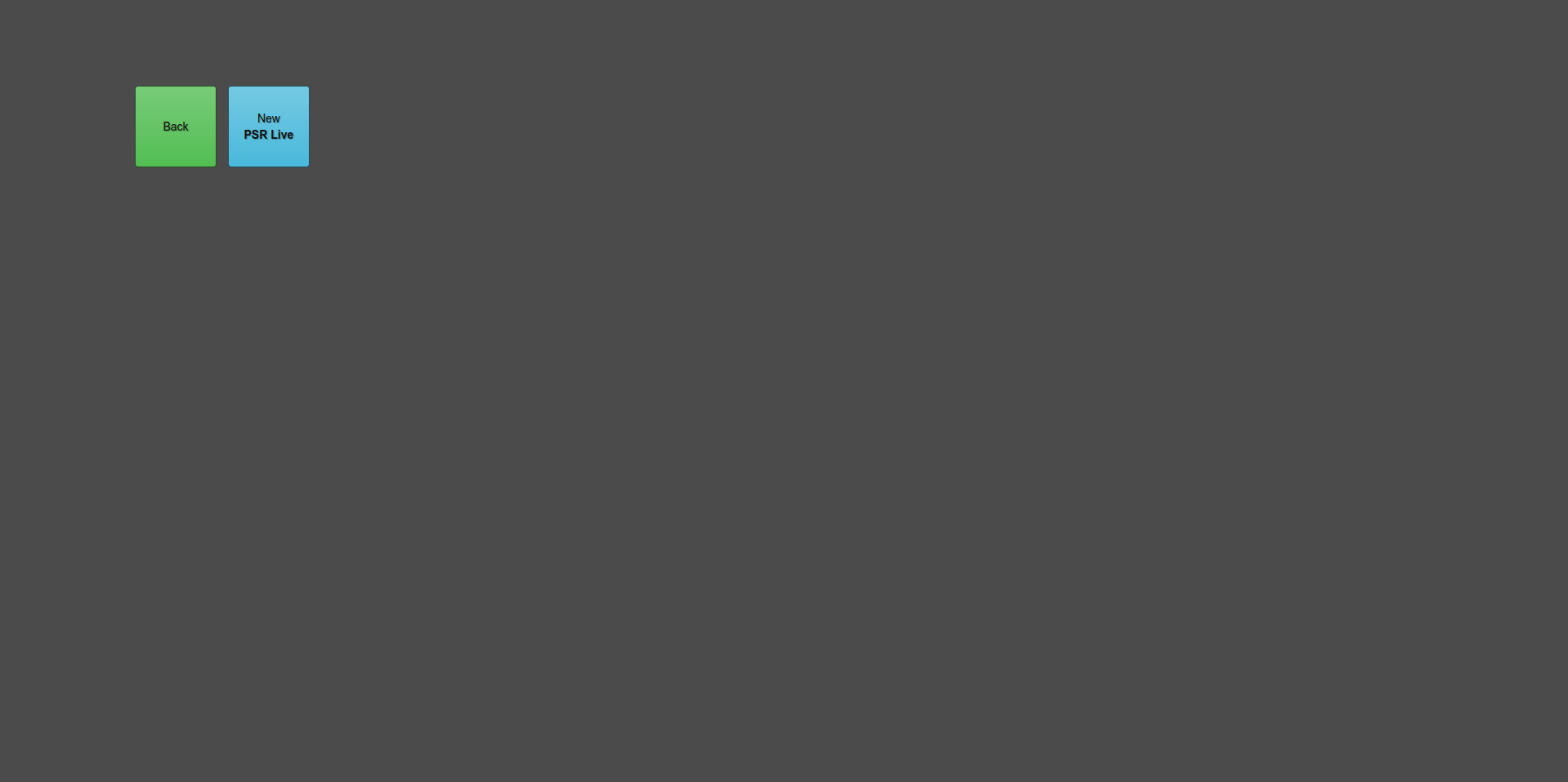
Click on the Icon to open it.
Now start dragging panels into FreeScope’s Workspace. On the top left side you can choose the panels. Just arrange them in a way that best suits you. If you have two or three screens, you can even drag the browser-window across several screens and create more space
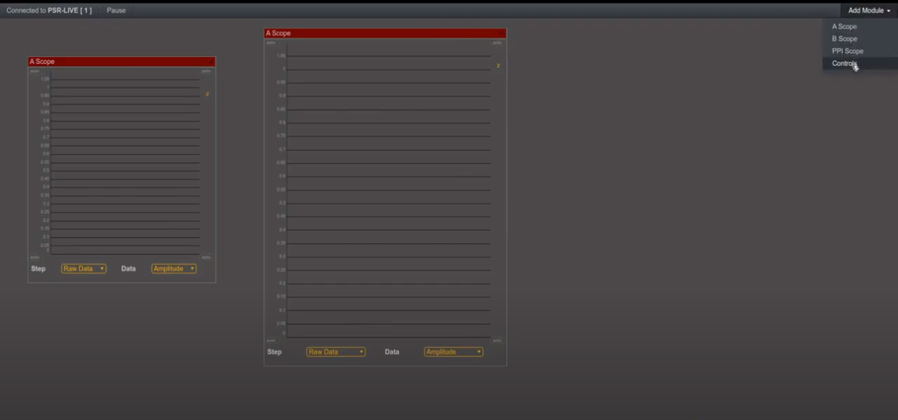
Try to mix various scopes. Try to use them intuitively.
Try to change the scale in the A-Scopes or the contrast in the PPI.
Get a “feeling” of the available controls systems.
When the controls are activated, they appear in the order as displayed in the control panel:
1) Suppress DC 2) Reverse Signal 3) STC 4) MTI 5) CFAR
2. Suppressing DC
2.1 Abstract
A strong source of noise, meaning a disturbing noise spectrum is the radar source itself. It is commonly referred to as DC (or D.C.). The amplitude of the radar source is so strong that - if we want to show its complete magnitude - it forces us to choose a bigger scale for the Y axis. Consequently, the targets which we want to focus on appear as very small peaks and might even get lost among the noise. So it is always a good idea to get rid of this amplitude from the beginning.
2.2 Performance Indicators
- Learners will be able to understand and interpret the spectrum of noise around the source seen in various scopes
- Learners will be able to apply means to suppress the D.C. source
- Learners will be able to identify the most suitable range calibration to receive the best image after suppression of the source.
- Learners will be able to understand and interpret the results indicated in the different scopes
2.3 System Set up
The radar will be placed on the rotary tripod. The tripod will be rotating, best looking at targets in 3-10 m distance.
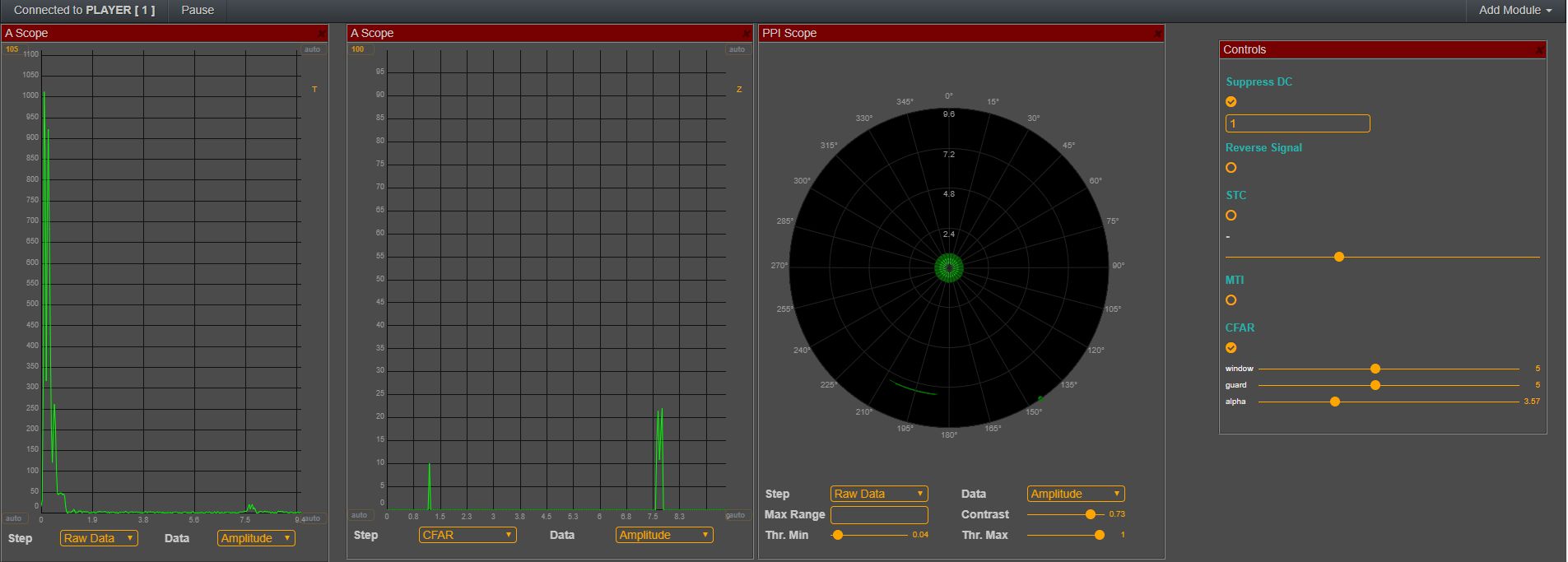
We will chose the A-scope, the PPI-scope, and the Control Panel
2.4 Experimental Procedure
Place one or more targets around the radar source. Actually you may also consider objects in your classroom and even the walls as targets. Just measure the distance of some characteristic targets (like the classroom wall, a desk, your computer etc.).
Place one target (e.g. a sphere) at a distance of 3 - 8 m to start off.
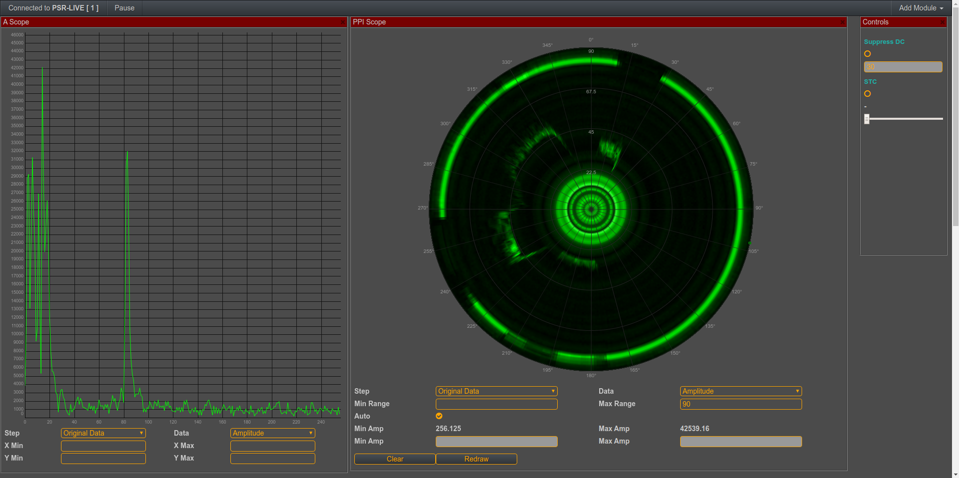
Place the A-Scope to the left, the PPI in the middle and the control panel to the right.
You can have the radar rotate immediately or start with a non-rotating radar. Get a feeling of what you consider easier for the calibration of your radar. Discuss with the other students and your teacher.
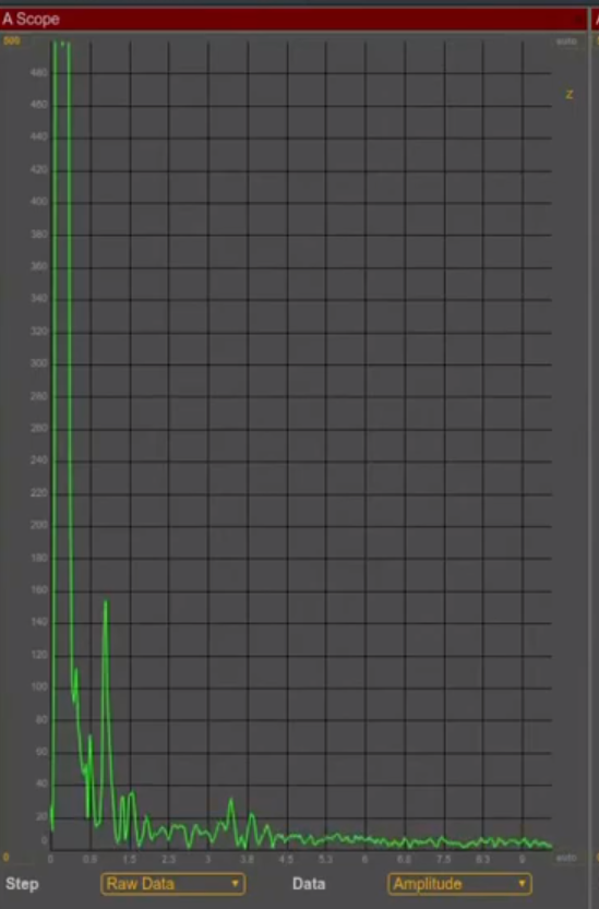
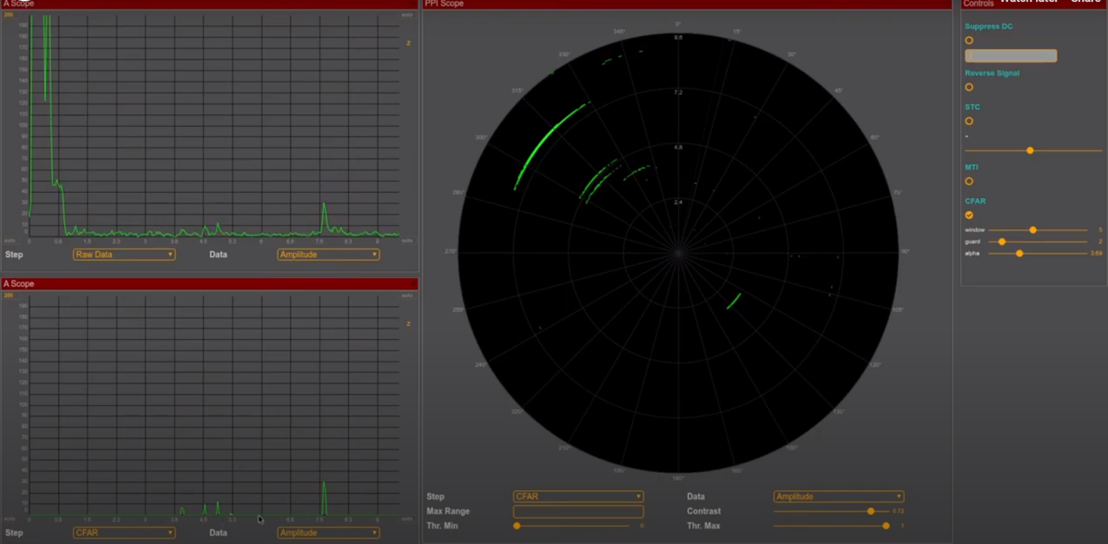
The radar image in A-Scope and PPI scope are dominated by the strong amplitude around the source. Relative to that reflection, all other targets appear small.
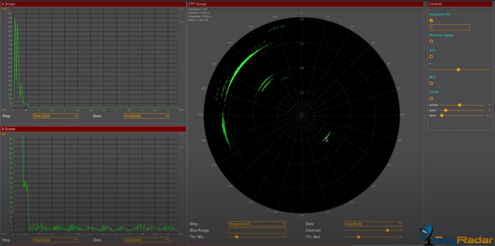
Step 1: In the control panel, you see the tick-box “Suppress DC”. That tick box will allow you to subtract the reflections around the source.
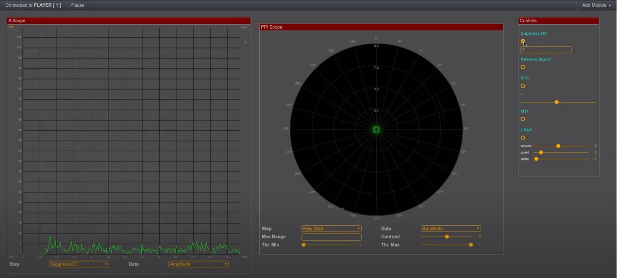
Step 2: You now adapt the scale of the y-achsis. You can click on it and define the maximum value of the amplitude. The absolute value on the Y-axis is specific to each radar source. The amplitudes and their visibility are important. Let us ignore the absolute value for now.
Try to choose a scale that gives you a good view of the targets.
You may also want to reduce the range on the x-axis (meters). That allows you to focus more on the targets in your near range. It also gives you the possibility to get rid of strong unwanted reflections like the walls of your classroom. In short, you may focus your attention on your range of interest.
Step 3: Let us now look at the PPI Scope. Just to see the impact of the source, you can shortly untick the suppress DC checkbox. You will see the circle around the center that is created by the noise spectrum of the source. Now let us take it off again.
After setting Suppress DC, give the system time to autoadapt. As it will autoadapt on the maximum values, it probably starts with an overdriven radar image, as it might only see "noise". This will change when it gets to the first real target. Then it adapts the image on this new maximum value. After one rotation, the autocalibration is done.
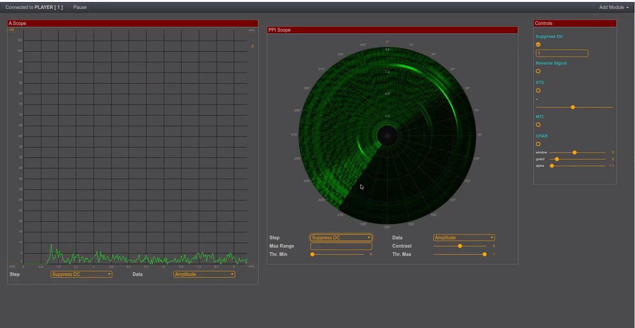
Use two tools to improve the visibility of your targets:
- play with the contrast of the PPI. Play around with the sliders and find the right compromise between an increase / decrease of noise on the radar image and a weakening of the reflection of the targets.
- Like in the A-Scope, optimize the range of your PPI on your area of interest.
Discuss the results with your colleagues and the teacher.
You might not be totally happy. To get better images, you will learn to apply the Threshold function, the STC and CFAR.
3. Sensitivity Time Control / STC Filter
3.1 Abstract
Reflections of closer targets are evidently stronger than the more distant reflections and give a wrong impression of originating from a bigger target. The STC function has the goal to attenuate reflections in the near range to lessen their visual dominance.
The STC function has the goal to attenuate reflections in the near range.
In this exercise we will try to bring the signal strength of a sphere in a distance of 2 meters to the same level then a sphere in a distance of 8 m.
Students can play with the magnitude of the STC slider and then observe the effect in FreeScopes.
3.2 Performance Indicators
- Learners will be able to understand and interpret the relation between STC and the impact on the radar images in the scopes.
- Learners will be able to calibrate the STC settings to receive a good radar image.
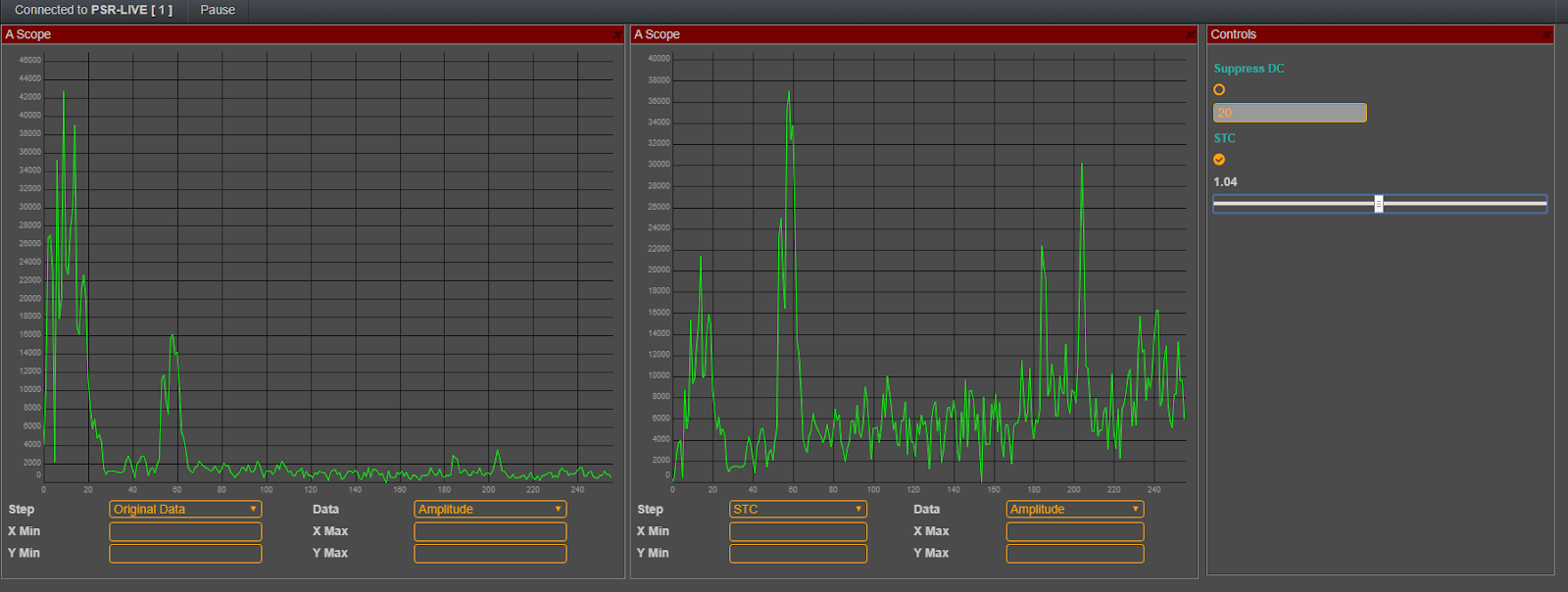
3.3 System Set up
The radar will be non-rotating, and looking at targets in 2 - 8 m distance. We prepare the FreeScopes with two A-Scopes and one control panel.
In the first A-Scope we show the Raw Data, in the second A-Scope we show the signal after STC.
3.4 Experimental Procedure
In the control panel the student will activate STC and adjust its value with the settings box. The curve will adapt, the near range objects will be weakened.
Now we can get the same image with the PPI-Scopes. So let us replace the A-Scopes with PPI-scopes.
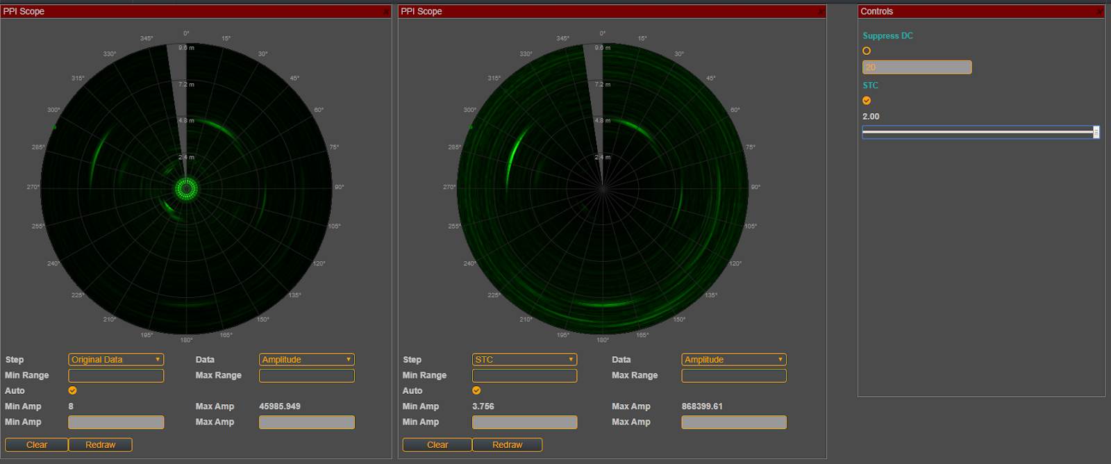
Applying what you learnt in the previous exercise and suppress the DC. Also play with contrast in the PPI. You can also play with the range. Try to position your focal targets in the central area between the source and the outer circumference of the PPI.
4. Threshold Function to Reduce Noise
4.1 Abstract
When looking at radar scopes, we have to minimize unwanted echoes to clearly see our targets and to avoid misinterpretations. Otherwise we might see targets that do not exist or have our targets hidden in unwanted echoes.
Let us in a first step try to understand the radar echo.
It consists of the reflections from our targets of interest, noise from our receiver and atmospheric noise, interferences from other radars or jammers, and clutter.
The term “clutter” is used for unwanted echoes in the radar scopes. Such echoes are typically returned from ground, sea, rain, animals / insects, chaff and atmospheric turbulences, and can cause serious performance issues with radar systems. In our classroom clutter comes from unwanted reflections of all the objects in the room.
We will look at the reduction of clutter later in this manual, when we reduce its impact with the help of Moving Target Indication, or simply MTI. But we will also learn how to eliminate unwanted reflections through the limitation of our observation window (excluding for instance unwanted reflections from the walls).
A simple means to reduce noise is a threshold which eliminate small echoes from the scopes.
4.2 Performance Indicators
- Learners will be able to understand and interpret the relation between the upper and lower threshold (Thr. and the impact on noise and consequently on the clarity of the images in the scopes.
- Learners will be able to calibrate the gain to receive a good radar image.
4.3 System Set up
The radar will be non-rotating, best looking at targets in 3-10 m distance.
4.4 Experimental Procedure
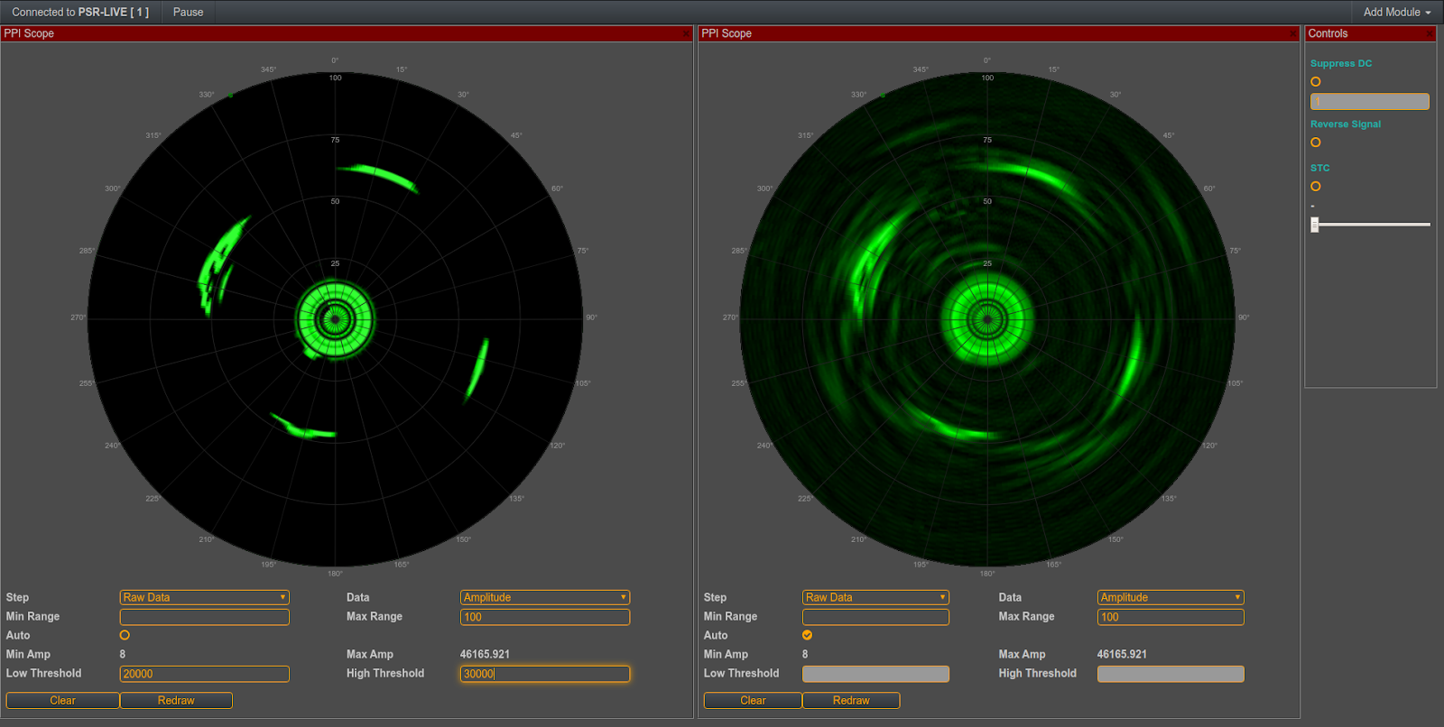
Using Threshold control limits noise. It also can be used to take out the upper spikes in the scopes.
Place an A-Scope and a PPI into your FreeScopes workspace.
To reduce the upper limit, change the high threshold in the box below the scope. This will help you to reduce the impact of unwanted reflections like the classroom walls.
To eliminate the noise, play with the lower threshold. This helps you to free your desired targets from disturbing echoes.
The absolute values of the amplitudes are again depending on the radar source.
Try deck out the desired targets to make them clearly visible
Apply also what you learnt in the previous exercises: suppress the DC and apply STC. Also play with contrast in the PPI. You can also play with the range. Try to position your focal targets in the central area between the source and the outer circumference of the PPI.
5. B-Scope and Threshold
5.1 Abstract
When the receiver is saturated, then the contrast of the B-Scope is decreased. You can show this effect with the threshold control and show all objects of interest without disturbances.
5.2 Performance Indicators
- Learners will be able to understand and interpret the relation between receiver’s saturation, gain and threshold and the impact on noise and consequently on the clarity of the images in the scopes.
- Learners will be able to calibrate the threshold to receive a good radar image.
5.3 System Set up
The radar will be non-rotating, best looking at targets in 3-10 m distance.
5.4 Experimental Procedure
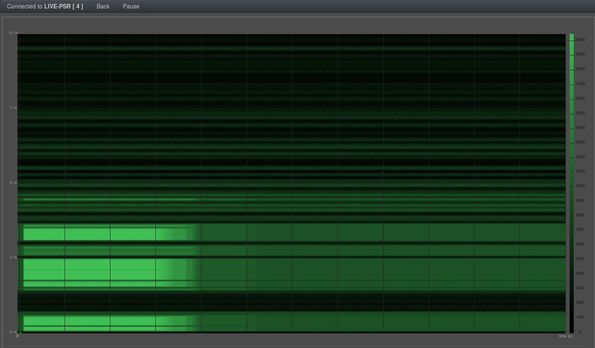
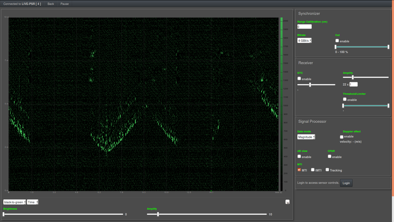
Use the B-Scope in time based mode. You’ll see this picture.
Change the high Threshold to a lower value, and see how it affects the contrast in the B-Scope.
When using the radar source in rotating Mode, you’ll see the same effect on the PPI-Scope.
6. A-Scope and I-Data and the MTI
6.1 Abstract
MTI (Moving Target Indication) is a strong means to distinguish moving objects from clutter. This intelligent algorithm simply erases all statis reflections from the scope, leaving you with a clear image of the moving target(s).
In this exercise we use the A-scope and the input mode “I-Data” for demonstrating the influence of moving objects. On the A-Scope you can see the alternating phase shift of the echo signal caused by the Doppler Frequency.
6.2 Performance Indicators
- Learners will be able to understand and interpret the relation between Doppler effect, I-Data and the representations on the A-Scope.
- Learners will be able to set the I-data to receive a good representation in the A-Scope.
6.3 System Set up
The radar will be non-rotating, best looking at targets in 3-10 m distance.
6.4 Experimental Procedure
Place an A-Scope Panel and the control panel into the freescopes workspace
Your desired target is the rotating fan. To remove all data, you’re not interested in, you can set the low and the upper threshold accordingly. All Data outside your defined observation window will not be displayed. Then activate the function MTI. Now you’ll see only moving targets.
When the fan is rotating with high speed, you won’t see much changes. After switching the fan off, you’ll see the phase change on the scope. It does not matter which data mode has been selected.
When you compare the two pictures above, you’ll see the phase change during the period where the fan is rotating slowly.
7. Moving Target Indication MTI
7.1 Abstract
The phase shift, analyzed in the previous exercise can be used for measuring speed, or for simple Moving Target Indication (MTI).
The Remote Controlled Quadcopter is a simple moving target. It does not need to fly in every case. It is also sufficient when the target is located somewhere in the class room and slowly turns its rotors only.
7.2 Performance Indicators
- Learners will be able to understand and interpret the relation between Doppler effect, I-Data and Moving Target Indication
- Learners will be able to apply Moving Target Indication to identify and track moving objects.
- Learners will be able to set the I-data to receive a good representation in the A-Scope.
7.3 System Set up
The radar will be non-rotating, best looking at targets in 3-10 m distance.
7.4 Experimental Procedure
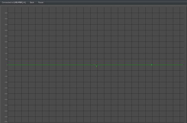
For this experiment you need a moving target. A human is reflecting the rays at 8 GHz or 24GHz very well. Without movement you’ll see a screen like this one:
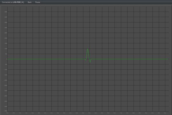
A moving human as target looks like this:
When the cross section is moving down in the scope, the object is moving towards the radar. When the target is moving up, it means the object is moving away from the radar.
8. CFAR
8.1 Abstract
In this exercise we use the A-scope and in a 2nd step the PPI. We compare the signal filtering capabilities of the dynamic CFAR in comparison to the static threshold control.
CFAR dynamically adapts to the constellation of noise and targets at each specific point. It uses a sliding window around a target, which calculates the mean value of neighboring reflections to determine the threshold for a specific cell under test. There are various variants of algorithms for the detection of the false alarm rate. We used the perhaps most common version. It has the following parameters:
- alpha - defining the threshold for the probability of false alarm (pfa) and detection (pf)
- window - the size of the observation window to estimate the noise floor (noise power)
- guard cells - they are the cells around the CUT which we ignore because of side-lobes from the target.
8.2 Performance Indicators
- Learners will be able to understand the difference between a static threshold and a dynamic CFAR.
- Learners will be able to clean the radar image optimized on specific targets.
8.3 System Set up
In the first experiment, the radar will be non-rotating, best looking at targets in 3-10 m distance. In the 2nd experiment (using the PPI), the radar will be rotating
8.4 Experimental Procedure
Experiment 1
In the first experiment, arrange three A-Scopes on a screen, and the control panel.
Let the radar look at several objects of different sizes, e.g., at a distance of 4m, 8m and 10m.
Set the first A-scope of raw data, the second on threshold and the third on CFAR.
Try now to optimize the setting of threshold and CFAR so that you see all targets.
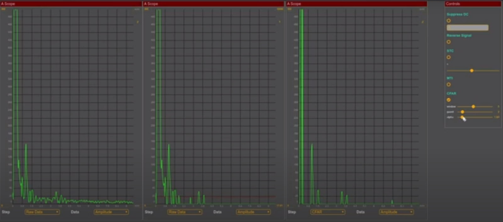
You will see that the CFAR is much better so catch small targets which are lost in the threshold.
You can find more guidance in the video
https://www.skyradar.com/blog/skyradar-nextgen-8-ghz-pulse-comparing-threshold-limiter-with-c-far
Experiment 2
In the 2nd experiment we arrange 2 A-Scopes and one PPI. Keep the first A-Scope on Raw Data, the 2nd on CFAR, and the PPI on CFAR as well.
Increase the contrast on the PPI to get a better image.
Let the radar rotate. Typically a classroom or laboratory offers many targets. If you work in a bigger lab you may place some targets across the room. Make sure you place smaller and bigger targets and various distances.
Now try to discriminate the targets against noise. It requires a bit of feeling and some playful optimization of the parameters of the CFAR.
When done you might try to see whether you get the same result with the threshold. You could also place two PPIs next to each other and operate one on threshold and the 2nd one on CFAR. Try to get the same results with both filters (it will be pretty impossible with the threshold as it does not adjust the settings on each targets).
You may want to look at article:
9. Radar Cross Section RCS
9.1 Abstract
The exercise provides a simple experimental set-up on how to measure the cross section of a radar. The size of the radar cross section is defined by the following parameters (source):
- the target\'s material
- the size of the target relative to the wavelength of the illuminating radar signal;
- the absolute size of the target;
- the incident angle (angle at which the radar beam hits a particular portion of the target, which depends upon the shape of the target and its orientation to the radar source);
- the reflected angle (angle at which the reflected beam leaves the part of the target hit; it depends upon incident angle);
- the polarization of the transmitted and the received radiation with respect to the orientation of the target.
9.2 Performance Indicators
- Learners will be able to understand the concept of a radar cross section.
- Learners will be able to measure a radar cross section.
9.3 System Set up
The radar will be rotating, best looking at targets in 3-10 m distance.
Place 1 or 2 A-Scopes and a PPI Scope on the screen. Let the radar rotate. Place a sphere as a target in a distance of 7-10 m in front of the radar.
9.4 Experimental Procedure
Calculate the cross section of the sphere you placed in front of the radar mathematically. Now try to get the same RCS. Simply click on the representation of the target in the PPI. FreeScopes will display the RCS on the upper left side of the PPI.
You may have a look at the video:
10. Parabolic Reflector and the Effect
10.1 Abstract
The parabolic reflector forms a fan beam pattern. The quadcopter can be used to show the dimension of the cone of silence of the PSR. In this demonstration the radar may better work with stopped antenna.
10.2 Performance Indicators
- Learners will be able to understand and interpret the effect of the parabolic reflector .
- Learners will be able to detect the cones of silence in a radar.
10.3 System Set up
The radar will be non-rotating, best looking at targets in 3-10 m distance.
In this experiment, the B-scope uses the time mode in the x-axis
10.4 Experimental Procedure
For this experiment you need two persons. One person is operating a drone and is trying to hit the beam. You can use any off-the-shelve remote controlled helicopter or quadcopter. You might increase its reflection if you cover it with aluminum foil. The other person observes the Scopes and corrects the settings during recognizing the cross section. As done in the lessons before, you should use all useful functions to get a better radar image (STC, CFAR, contrast). You have to find the ideal settings to capture the drone. So best focus on the position of the drone in the scopes. After this lesson you’ll understand the difficulty to operate a radar with a small beam in non-rotating mode.