


When it comes to radar, the FFT (Fast-Fourier Transform) is used to convert time domain signals into frequencies. An example of its use is for converting the dual channels of a pulse-Doppler radar from time domain into range-Doppler data.
A typical signal reflected back from an object to the radar may look like the one in Figure 1 when digitized by the radar’s analog-to-digital (A/D) board. The A/D board converts RF signals into digital signals for processing. If we take an FFT of this signal, the result is plotted in Figure 2. The question often asked is, “Why is the FFT plot of a pulse-Doppler Radar mirrored?
The answer is that it isn’t mirrored. One half of the plot are the negative frequencies, and the other half of the plot are positive frequencies (see Figure 3). To make the plot more understandable, we need to reorder the indices on the x-axis. Figure 4 shows Figure 2 replotted with the reordering of indices shown in red. As you can see in this plot, the mirroring is gone and a strong response is plotted in the center of the graph.
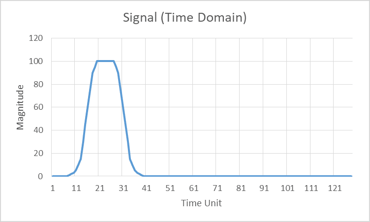
Figure 1. A radar signal in the receiver after demodulation has been applied.
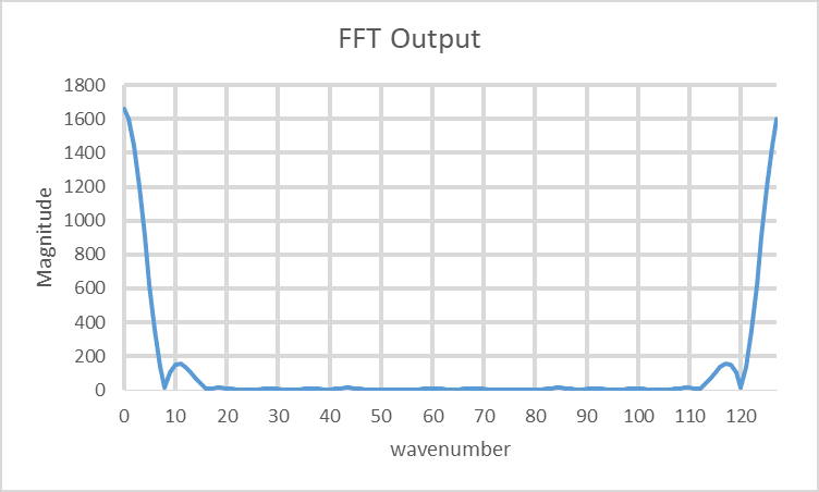
Figure 2. This is the FFT plot of the signal in Figure 1.
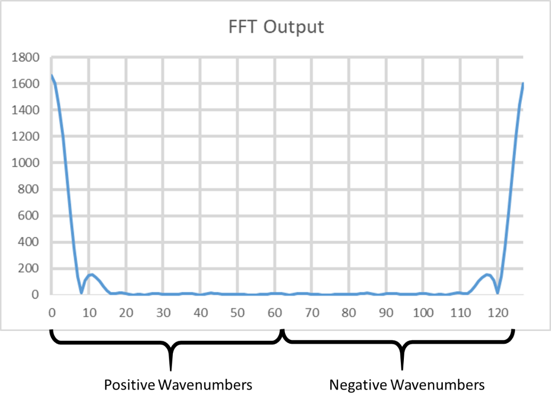
Figure 3. The FFT plot explained. Although indices are linearly increasing, their representation of the data is counterintuitive.
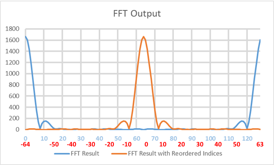
Figure 4. By reordering the indices, the red line above represents the typical representation of an FFT plot of a radar signal. Note that the red numbers under the x-axis are the new ordered indices.
For a pulse-Doppler radar, the indices may be combined with the PRF (Pulse Repetition Frequency) and the transmitted frequency to supply velocity on the x-axis of these plots. Velocity is a vector, so negative speeds means the object is going away from the radar, and positive speeds mean it is coming toward the radar. PRF is the number of pulses transmitted from a radar per second.
To convert the x-axis wavenumbers to Doppler velocities, we need to first compute the maximum unambiguous speed of the radar. The maximum unambiguous speed of a pulse-Doppler radar is computed by the formula:
Max Radial Velocity (m/s) = Vrmax = C * fPRF/(4*fTX),
where C = speed of light (m/s),
fPRF = PRF (Hz)
fTX = transmitted frequency (Hz).
Once this speed is computed, we can compute the Doppler resolution for the radar using the formula:
Doppler Resolution (m/s) = Vrmax/(number of pulses integrated/2).
A pulse-Doppler radar integrates pulses over time to compute the Doppler velocities. It also results an integrated power that is substantially higher than a single pulse. The new x-axis is created by multiplying the reordered indices by the Doppler resolution as shown in Figure 5.
Figure 5 was plotted assuming a radar with a transmitted frequency of 10 GHz, a PRF of 4,000 Hz, and 128 pulse-integration. Using the equations above, Vrmax = +/- 30 m/s, and the Doppler resolution = 0.46875 m/s.
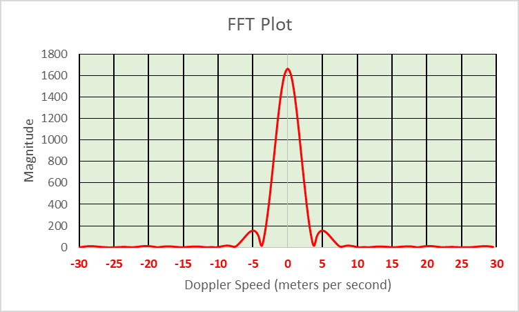
Figure 5. Using PRF and transmitted frequency, the indices can be converted into Doppler velocity.
Meters per second is not commonly used for a measurement of speed, so we can use the conversion Vkph=(Vmps /1000)*3600. Figure 6 is the same plot as Figure 5, but with the x-axis converted to kilometers per hour (kph).
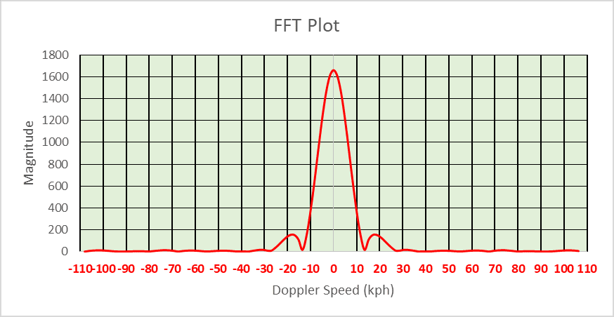
Figure 6. This is the Doppler plot from Figure 5 with the x-axis converted to kilometers per hour.
As stated earlier, the maximum speed that can be measured by the pulse-Doppler radar in this example is +/- 30 m/s, which is +/- 108 kph. What happens if an object is moving with a radial velocity (a velocity that is toward or away from the radar) that is greater than 108 mph? Its speed will wrap around to the negative side of the plot. This is why the term “unambiguous speed (or velocity)” is used for these maximums. Radar designers should be careful to design their radar systems so that the object of interest will appear within these maximum bounds. To combat the problem of detecting objects with ambiguous speeds, the radar designer can increase the PRF rate or lower the transmitted frequency. Since the transmitted frequency is harder to change once a radar has been built, it is easier to change PRF.
In Figure 6, we see that the object’s signature is spread across 0 Hertz. In this particular case, it is because the signature was finite in Figure 1. It is the artifact of taking the FFT of a finite signal. The wider that signal is in Figure 1, the narrower the signature will be in Figure 6. But there can be other reasons for the spread in the signature of a pulse-Doppler radar. These include:
- The object is swaying or has parts that are moving relative to main body. If the person is swaying or their arms or hands are moving, the signal can spread across adjacent Doppler cells at zero Doppler. This can be seen with trees whose branches are swaying in the breeze.
- The reflected signal off the object can be so strong that it saturates the radar receiver. Think of saturation as drinking water from a garden hose at full force. You can't drink fast enough, so you lose water to the ground. The same is true with radar. The received signal is so strong that it exceeds the radar's ability to consume all of it. The signal is clipped, which means information concerning the signal is lost. This results in a Doppler spread around the main body signature when passing through the FFT.
- A failure of a component in the radar can result in Doppler spreading and many other artifacts in the FFT plot. For instance, if the radar loses coherency (typically resulting from a failed component such as the Local Oscillator), then the Doppler signal can spread or truly mirror on both sides of the plot.
Regardless of the reason for Doppler spreading in the object's signature, you will see the spreading blob at both ends of the spectrum for a slow moving object if you forget to reorder the indices. If you have properly reordered the indices, you will see this as a single blob in the center or near the center.
Another Example of Mirroring:
Figure 6 represents the Doppler signature of an object at a given range. The plot could be converted into a single row of colored boxes as shown in Figure 7. In this figure, there are 16 pulses used for the FFT, which results in 16 columns. The magnitude of Doppler is represented in color. There has been no reordering of the indices in Figure 7, so the signature from a slow moving object will appear at the outside edges of the plot, as shown in the in Figure 8. Reordering the indices will be allow the Doppler signatures for a slow moving object to appear in the center (see Figure 9). Additional rows of boxes can be stacked, which represents increasing range going up. This is shown in Figure 10, and is commonly referred to as a Range-Doppler Plot.

Figure 7. The FFT plot can be also represented as a row of boxes, where signal strength is represented by color.

Figure 8. This shows an object has entered the range monitored by the radar. The red color boxes of the non-reordered plot indicate the object is almost stationary.
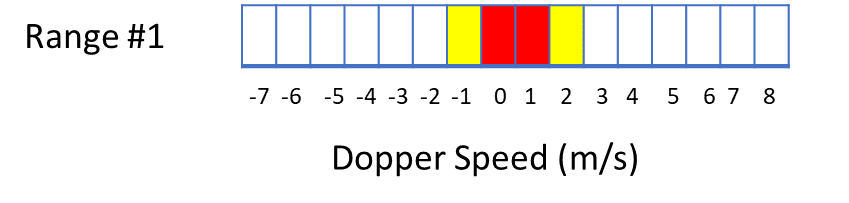
Figure 9. This is Figure 8 after the indices have been reordered and the Doppler frequency is converted to speed.
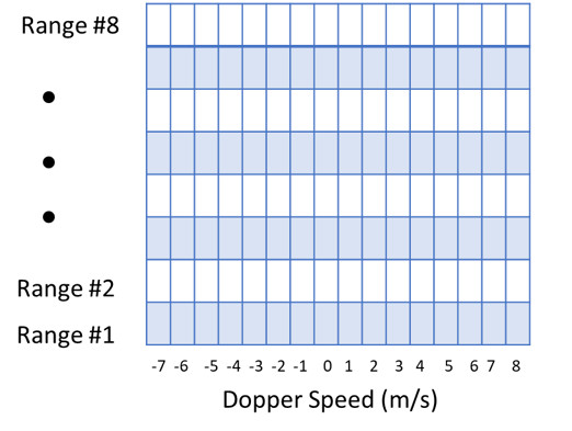
Figure 10. This is a Range-Doppler Plot. Doppler velocity is supplied for each range.
Watch this video of a Range-Doppler Plot of a human walking outdoors:
Figure 11 is the Range-Doppler plot from an X-Band radar designed to detect humans.

Figure 11. The top graph is the peak Doppler signal seen from 0 to 65 meters from the radar. The bottom plot is the range-Doppler plot, which is also known as a Doppler Time Intensity Plot.

Glossary (Terms used in the text):
Pulse Repetition Frequency (PRF): The rate at which pulses are transmitted in a radar per second.
Doppler: The change of frequency caused by motion from an object. The emitted frequency from a radar transmitter is shifted upwardly if the object is moving toward the radar, and downwardly if the object is moving away from the radar.
Doppler Resolution: This is the smallest increment of speed that the pulse- Doppler radar can detect. A radar that is trying to detect people movement will have Doppler resolutions of a few centimeters/second.
FFT Plot (Range-Doppler Plot): The FFT is used to convert radar time domain data to frequency domain. Detected objects and their Doppler signature are plotted in an FFT Plot. The x-axis represents the Doppler Frequency (which can be converted to Doppler Speed), and the y-axis is range. The Range-Doppler Plot is also referred to as the Doppler Time Intensity Plot, especially if it is recorded as a data stream.
Magnitude: This is the signal strength. In the plots of this paper, the units were not specified, but are commonly supplied in voltage or in power.