Artificial Intelligence: Hidden Markov Model Classifiers and RADAR Objects Classification by Machine Learning 1/2

In this article we will explore a very special class of classifiers, the Hidden Markov Model Classifiers (HMMs). They are mainly a statistical and probabilistic model but they have found their entry in the world of Machine Learning since they can be trained and classify data.

They found a natural use for the automatic recognition and inherent classification of RADAR objects since these objects are obtained by sampling time-dependent data. The concept of Hidden Markov Model classifier is not straightforward and necessitate the prior knowledge of several other concepts:

• Bayesian probabilities
• Bayesian naive classifiers and Bayesian Networks
• Markov processes

We will go successively through each of these concepts in a very synthetic way so to give the reader an understanding of the inherent logic behind such classification techniques. 

Bayesian Logic

Bayesian probabilities are conditional probabilities. They are a part of the Bayesian statistics named after their inventor, the mathematician Thomas Bayes (1701 - 1761). 

The core principle is to compute the probability of an event knowing that another event has occurred. In other terms Bayesian probabilities explain how to compute the probability of A when you know that B with a probability of P(B)has realized, this is contained in the following formula (Bayes theorem) :

P(A|B) = P(B|A) * P(A) / P(B)

The formula reads literally “The probability of A to realize knowing that B has realized is equal to the product of the probability that B realizes knowing that A has realized by the probability that A realizes divided by the probability that B realizes”

That simple formula is a powerful engine to compute a lot of useful things in plenty of domains.

There are a lot of literature about Bayes Theorem in different forms, here we wish only to present what is needed for the reader to understand the Bayesian classifiers.

We are here interested in the Bayesian interpretation of the theorem:

P(A) represents the prior. That is to say the a priori belief that event A is true/ event A will realize.

P(A|B) represents the posterior, that is to say the belief A is true/A will realize taking the support that provides B into account. 

P(B|A ) / P(B) represents the support B provides to A. if that support is <1 then the support is negative, e.g the belief is A is lessened otherwise it is a positive support, the belief in A is enforced.

The Bayesian interpretation is the root of the Bayesian machine learning. This consists in believing some facts are true giving (anterior) facts realized.

We give here one example of the power of Bayesian probabilities which often provides paradoxical solutions because our human brains evaluate in general very poorly such conditional probabilities.

Bayesian rule is often used in genetic engineering and in general in medicine. It is often a powerful tool for a doctor to make an opinion of take a decision.

A typical example of Bayesian logic

A particular virus has a base rate of occurrence of 1/1000 people. This means that on average 1 person over 1000 in the population will be affected by that virus. 

It is essential to be able to detect the virus in the population before the incubation completes so to cure the infected people.

A governmental laboratory manufactured a test to detect that disorder. It has a false positive rate of 5%. This means that 5% of the time it says a given person has a disease, it is mistaken. We assume that the test never wrongly reports that a person is not infected (false negative rate of 0%). 

In other words, if the test says a person is infected there is a 5% chance it is incorrect but if the test says a person is not infected, then this will be always correct.

Before a decision to start testing the population and producing massively test kits, the doctor in charge of the fight against virus is asked by the authorities the following question: 

“What is the chance that a randomly selected person which have a positive result to the test is effectively infected by the virus?”

Most people would intuitively answer : 95% because as a matter of fact the test says wrongly that people are infected by the virus only 5% of the time.

The doctor being a highly trained specialist starts to use the Bayesian computations:

A is the event that a person has the disease.

B is the event that the person has a positive result to the test.

P(B|A) is the probability that a person which tests positive has the virus. This is what we need to compute.  For that we need to compute P(A), P(B) and P(A|B). 

It is easy to compute P(A) , this is 1/000= 0.001 (recall the virus infects on average one person over 1000 in the population) 

P(A|B) is the probability that a person which has the disease will test positively, as we said the test has a false negative rate of 0%, so P(A|B)=1.

P(B) is the probability that a person in the population has a positive result to the test. 

There are two independent ways that could happen:

• 1) The person has the disease

There are then a probability of 0.001 that a person has the disease 

• 2) The person has not the disease and triggers a false positive

There is a probability of 0.999 that a person has not the disease and  probability of 5%=0.05 that this person will trigger a false positive

Finally 

P(B) = 0.001 + (0.999) * 0.05 = 0.051

We can compute P(B|A):

 P(B|A) =  1 * 0.001 / 0.051 = 0.02

As a matter of fact the test will give on average correct results only 2% of the time, so it is highly inaccurate and an other test need to be manufactured!

The reality is that few people have the virus so the false positives even if they are “only” 5% are destroying the accuracy of the test but that fact is highly difficult for a human mind to apprehend.

Bayesian Classifiers : The Naive Bayes Classifiers

An application of Bayesian logic are the Bayesian Classifiers. The Bayesian classifier is a learning machine which uses a finite fixed set of outputs , the labels or categories where the inputs, unknown must be classified. To do this, the Bayesian classifier use Bayesian logic, that is to say the correction of the prior belief that such input will fall into such category given support from additional events or information:

posterior (A|B) = prior(A) x support from additional facts (B|A/B)

Which can be formulated as :

posterior = prior x likelihood / evidence.

Here we defined likelihood as p(B|A) and evidence as p(B).

First let us look as the most simple of all the Bayesian Classifiers , the “Naive” Bayesian Classifier. 

The main idea behind such classifier is that we are given at the start the following conditional probabilities:

P(C_k| X₁, ..., X_n) k=1, ..., m

Where C_!,...,C_m are the available categories and  X=X_!, ..., X_n is the input vector to classify.

We can write:

P(C_k | X₁, ..., X_n) = P(C_k) P(X|C_k)/P(X) k=1,...,m

The term P(X) is a normalizer constant in that sense that it does not depend on the m categories. P(C_K) is easy to compute, it is the proportion of the whole dataset which is classified in the category CK.We can compute P(X|Ck)by considering that it is proportional to the joint probability model P(X, C_k)  and then we may apply the following rule chain:

P(X, C_k)=P(X₁ `nnn` (X₂, ..., X_n, C_k)) = P(X₁|(X₂, .., X_n, C_k)) . P(X₂, ..., X_n, C_k)

k=1, ..., m

And then finally by iterating n times that chain rule:

P(X, C_k) = P(X₁ | (X₂, .., X_n, C_k)) . P(X₂ | (X₃, .., X_n, C_k)) ... P(X_n-1 | (X_n, C_k)) . P(X_n, C_k) p(C_k)

The components of X are supposed to be all independents and by the so-called “naive” hypothesis:

P(X_i | (X_i-1 , .., X_n, C_k)) = P(X_i|C_k)

Here we must explain two aspects:

1. It is not trivial why a conditional probability P(X|C_k) is suddenly “transformed” into a joint probability P(X,C_k) .
   In fact P(X,C_k) `hArr` P(X `nn` C_k) = P(C_k) . P(X|C_k) by the probability chain rule, so the both quantities - seen as depending only on X - are proportionals 
2. It is also not trivial what the “naive” hypothesis means and why it is called “naive”. 

The components of X are supposed to be all independents - this is where the naivety is, so as a consequence, the condition that we have a realization of a value for one of the components of X should not depend on the realization of the others components of X but only on the realization of the categories.

From there, we can compute our model:

P(C_k | X₁, ..., X_n) = `1/Z` P(C_k) . `prod_(i=1)^n`P(X_i | C_k)

k=1,...,m

And Z is a scaling factor equal to:

Z = P(X) = `sum_(k=1)^m`P(C_k) . P(X | C_k)

These equations are the basis of the “Naive” Bayesian classifiers which are among one of the most powerful classifiers that exists.

Usually the decision to classify, that is to say to create a mapping between the input vector X and one of the output categories will be done by the Maximal a Posteriori (MAP) but it can also be done via the Maximal Likelihood (MLE)

MAP decision making

We classify X as C_k such as:

F(C_k) = max_k F(C_k)

where:

F(C) = P(C) . `prod_(i=1)^n`P(X_i | C)

MLE decision making

We classify X as C_k such as:

F(C_k) = max_k F(C_k)

where:

F(C)= `prod_(i=1)^n`P(X_i | C)

Both approaches have their pros and cons. MLE and MAP are widely used techniques in machine learning.

Bayesian classifiers may use naive models but with the assumption that the probability
P(X |C_k) will follow a normal distribution. The normal distribution is then computed by the estimation of the mean and variance parameters from each category in the existing dataset. Same may be done with multivariate Bernoulli and other probability laws.

Limits of the “Naive” hypothesis

The “naive” assumption that there is independence of the vector data of the input X is often, in many applications,  unrealistic Therefore to tackle that problem, Bayesian networks were invented.

The principle is to represent relationship between the vector component of X, eg the Xi | Xj by a unidirectional arrow. Therefore a graph will represent the components P(Xi | Xj) which must be taken into account into the overall computations of the MLEs or MAPs.

General Bayesian Classifiers: Bayesian Network Classifiers 

Historically Bayesian Networks (BNs) were not considered as classifiers ( and hence could not be considered into the Machine learning category ) but since naive Bayes classifiers obtained surprisingly good results in classification, BNs became increasingly used as classifiers.

Bayesian networks do not suppose that the input parameters of a Bayesian classifier are independent from each other. Therefore the Bayesian system form a directed graph (network) where variables are linked between each others by conditional probabilities as well. 

We recall that a bayesian classifier takes n input parameters which forms an input vector characterizing an object X to classify among N candidates classes {C₁, ..., C_N} . For example X = (X₁, ..., X_n).

A naive Bayesian classifier achieves its goal by computing products known as Maximum Likelihood (MLE) or maximum a posteriori (MAP) which involves the knowledge of  P(Ck) k=1, ..., N and P(X_i|C_k) i=1,..,n.

A Bayesian network will require more complex computations involving the cross-probabilities P(X_i|X_j) (i,j) =1, ..., n. To visualize this, we draw the n variables and we connect them when they have a dependency relationship (e.g., they are not independent variables from each others )

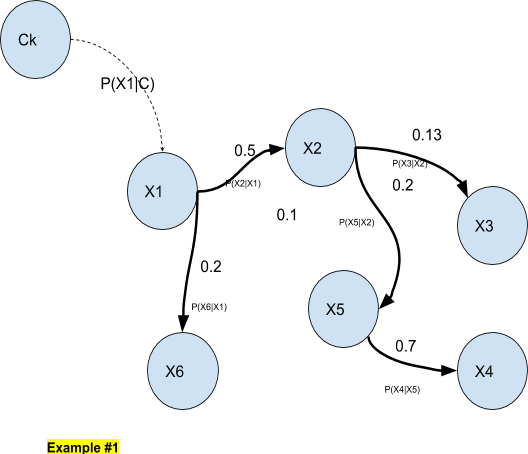
In the above example, we have a 6-dimensional input vector where variables are dependant of each other. 

The Bayesian networks are of course a most accurate model than the naive Bayesian classifiers but they require to be able to compute Maximum Likelihood (or similar products) , which may be a problem because of the cross-probabilities. 

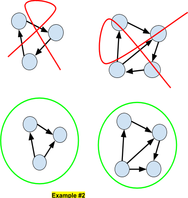
DAG

Bayesian Networks are Directed Acyclic Graphs (DAG) in the sense that it is impossible to connect two nodes by a path.  Here we show some examples of non-DAG (top) and DAG (bottom) networks. 

d-separated/d-connected

If A and B are two nodes in the graph and A and B cannot be connected by a directed arc, then A and B are said to be d-separated, otherwise they are said to be d-connected.

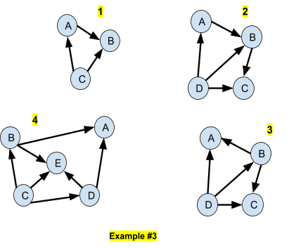
In the above 4 networks (Example #3), we have the following properties:

1. A,B and C are all d-connected between each others
2. A,B,C  and D are all d-connected between each others
3. A and C are d-separated
4. A and E are d-separated

Joint Distribution Model

Example

A Bayesian network always represents a joint distribution. In the above example (Example #1) with the 6-dimensional input vector, we have:

p(X₁, X₂, X₃, X₄, X₅, X₆) = p(X₆|X₁) p(X₄|X₅) p(X₅|X₂) p(X₂|X₁) p(X₃|X₂) p(X₁)

The log-MLE here is:

`f`(`theta`) =log `prod_(i=1)^n`P(X_i | X₁, .., X_i-1 ,X_i+1, ..., X_n, `theta` ))

And we look for a minimum of f over the classes to perform the classification.

In our example, the log-MLE will be:

`f`(`theta`) =log P(X₁| `theta` )+log P(X₂|X₁)+log P(X₃|X₂)+logP(X₅|X₂)+logP(X₆|X₁)+log P(X₄|X₅)

To classify the input we will pick the class `theta`  = `hat x` such that

`f`( `hat x`) = min_k=1...N `f` (C_k)

In the example, the class node is only connected to X₁ so that the maximization of `f`  consists only in the maximization of P(X₁| `theta` ).

General case

To compute the joint probability it is in fact quite simple, it is needed to get the products of all the CPDs, e.g., the product of the conditional probabilities of each X_i regarding to its parents in the network, P ar(i).

P(X₁, ..., X_n) = `prod_(i=1)^n` P(X_i | P ar(i))

We compute the joint probabilities in the 4 networks of Example #3:

The likelihood will be computed identically. Let us assume that there is a ‘universal’ node which connects to all the node of the network and which represent the category node. 

The log-likelihood will be:

`f` (`theta`) = log `prod_(i=1)^n` P(X_i | P ar(i), `theta`)

Therefore the classification of a sample (X1,..,Xn) will be done by picking up the category (or a category if there are several possible candidates) which maximizes the likelihood,.

The CPDs will be estimated by the samples of the training set. We give the value of the log-likelihood with the 4 networks of Example #3:

The problem consists in describing - and computing - the cross conditional probabilities, eg the probability distribution of X conditional from X’s parents,  from the training data.

The Bayesian distributions can be estimated from the training data by maximum entropy, for example but this is not possible when the network isn’t known in advance and has to be built.

In fact the complex problem here is to define the graph of the network itself which is often too complex for humans to describe it. This is the additional task of Machine Learning, besides the classification, to learn the graph structure.

Learning the Graph Structure

Here are the main algorithms used for learning the Bayesian Network graph structure from training data:

• Rebane and Pearl’s recovery algorithm;
• MDL Scoring function [1];
• K2;
• Hill Climber;
• Simulated Annealing;
• Taboo Search;
• Gradient Descent;
• Integer programming;
• CBL;
• Chow–Liu tree algorithm [2].

Overview of Different Bayesian networks

The main techniques of building specific classes of Bayesians networks are based on selecting feature subset or relaxing independence assumptions.

Besides this, there are improvements of the naive Bayesian networks such as the AODE classifier which are not themselves Bayesian networks, which is outside the scope of the present article. 

Tree augmented Naive-Bayes (TAN)

The TAN procedure consists in using a modified Chow–Liu tree algorithm over the nodes X_i, i=1,..,n and the training set, then connecting the Class node to all the nodes X_i, i=1,..,n.

BN augmented Naive-Bayes (BAN)

The TAN procedure consists in using a modified  CBL algorithm over the nodes X_i, i=1,..,n and the training set, then connecting the Class node to all the nodes X_i, i=1,..,n.

Semi-Naive Bayesian Classifiers (SNBC)

SNBC are based on relaxing independence assumptions.

Bayesian chain classifiers (BCC)

This is a special case of chain classifier applied to Bayesian networks. They are useful for multi-label classification, e.g., when classification may be multiple.

In this part we defined the concepts needed to understand the concepts of Bayesian Classifiers which are required for the comprehension of the Hidden markov Models Classifiers. Per se, RADAR objects can not be rightfully classified using Bayesian logic itself because RADAR objects are not time-independent statistics. A RADAR object is a collection of parameters which are varying over time and as such Bayesian logic itself poorly understands it. 

Bayes logic can classify, for instance, text data which are characterized by the probability of apparition of certain words as an inherent feature of such data. To classify RADAR data , it would be needed to take characteristic data such as an average speed, an average range, etc… While it is possible, the classification loose accuracy. 

Next

Fortunately it is possible to use a much more accurate method: the dynamical Bayesian network classifiers, also known as Markov Models Classifiers. This is what we will explain in the second part of this series.

References and Further Reading

• More articles on artificial intelligence (2019 - today), by Martin Rupp, Ulrich Scholten, Dawn Turner and more
• LEARNING ALGORITHMS FOR CLASSIFICATION: A COMPARISON ON HANDWRITTEN DIGIT RECOGNITION (2000), by Yann LeCun, L. D. Jackel & al, AT&T Bell Laboratories
• [1] Note that using MDL - aka minimal description length score -  (or any other ‘generic’ scoring functions) in order to learning general Bayesian networks usually result in poor classifiers
• [2] Chow and Liu algorithm finds the optimal (in terms of log likelihood minima ) bayesian network.