Artificial Intelligence: Hidden Markov Model Classifiers and RADAR Objects Classification by Machine Learning 2/2

In the first part of this series, we introduced the general concepts needed for understanding the Hidden Markov Models Classifiers. Namely: Bayesian Logic, The concept of Bayesian Classifiers and Bayesian networks. All these notions are now grouped to form a new type of classifier which can accurately model and classify time-series data such as the RADAR data.

What is a Markov model ?

A Markov model is a stochastic model designed to model systems which varies over time and change their states and parameters randomly (e.g., dynamical systems) . This can be for example:

• The price of a crypto-currency;
• Board games played with one or more dice;
• Some values from a stock market;
• The trajectory of a vehicle;
• Data from the weather of some given location (snow/sunshine/rain);
• RADAR data (our interest here!)

There are four types of Markov models:

• Markov chains,
• Markov decision processes,
• Partially observable Markov decision processes and
• Hidden Markov models.

Markov models relates to systems - Markov processes - where the future state is only dependent of the ‘most recent' values.

A stochastic process x(t_i), i=1,2... is said to be a Markov process is for every n > 0 and every numerical value y:

P(x(t_n) `<=` y | x(t_n-1), ..., x(t₁)) = P(x(t_n) `<=` y | x(t_n-1))

In other terms, the value of the state of the system at the instant T=tn only conditionally depends on the value of the state of the system at the previous instant T=t_n-1.

This property of the Markov model is often referred to by the following axiom:

‘The future depends on past via the present’. [9]

A Markov process with a finite number of possible states (‘finite’ Markov process) can be described by a matrix, the ‘transition matrix’,  which entries are conditional probabilities, e.g (P(X_i|X_j))_{i,j}.

As an example, we consider the Markov process created by the movement of an insect in the air - say a fly. The process has four states: “North, South, East, West” with the following (constant) conditional probabilities:

A Markov process is usually represented by a graph where the relations between the states are coded by connections.

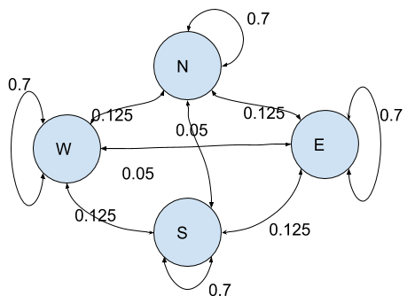
In our model, at any position, the insect have higher probability (70%) of keeping up with its trajectory, a small probability (5%) of going back where it came from and equal probabilities or turning left or right (12.5%).

If P is the transition matrix, then the transition matrix from a state at T=t_n to a state at T=t_n+k is given by the new transition matrix Q=P^k.

The above model is a Markov chain model because it is fully observable. Not all models have such properties, instead often the Markov model is hidden from observation and is known to the observer only via side-events.

In this article, we are only interested in the latter, the Hidden Markov models (HMMs). They occur for autonomous systems which states are partially observable.  In the case of the example with the insect, the hidden model would be the nature of the flying insect ( fly, mosquito, dragonfly…) and the observable model would be the directions taken by the insect.

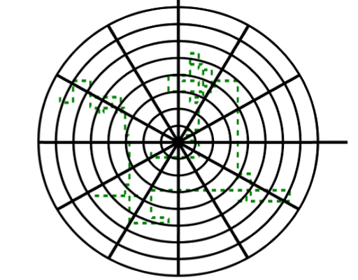
As an example, we display the trajectory of such an insect with 300 RADAR ‘spots’.

Next we display an example of such insect trajectory with 2,500 spots :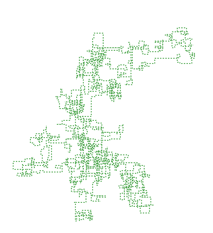A HMM classifier would have to decide the nature of the moving flying insect (hidden model) from such trajectories (observable model). 

It would be trained by a set of known classified trajectories obtained from existing dataset. 

Overview of Hidden Markov models

In a hidden Markov model (also named Labelled Markov Chain) , the Markov chain - itself - is hidden (X_i), only we see observable events (E_i) depending on the states of the Markov chain. Note that in Hidden Markov models, variables are discrete and not continuous. The continuous version of HMM is named the linear-Gaussian state-space model, also known as the Kalman filter, not to be considered here.

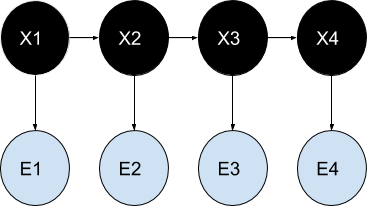
In terms of classification/recognition this means to be able to classify information given a series of ‘characteristic’ observations. For example, we could classify a moving insect(Xi) knowing only its trajectory(Ei).

Per se, hidden Markov models are not Machine Learning algorithms at all. They are a probability model and bear no information on how to learn, how to be trained and how to classify, so they need in addition algorithms to do so. Hidden Markov Models are usually seen as a special type of Bayesian networks, the Dynamical Bayesian networks.

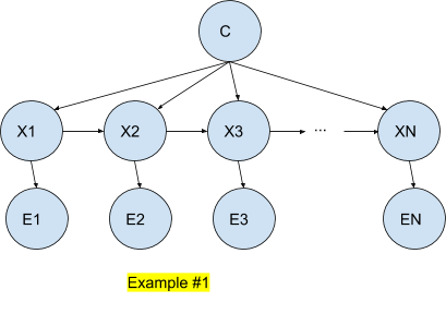
In such a model, the input vectors are N values of the observable model  (among n possible states in the finite case) .The Bayesian network is simplified regards to a general Bayesian network since every node (X_i) has (X_i+1) and C - the category node -  as parents.

In the above example, we can express the joint probability as such:

P (X₁, ..., X_N, E₁, .. ,E_N) = P (X₁) P (E₁|X₁) `prod_(t=2)^N`P (X_t|X_t-1) P (E_t|X_t)

This can be easily checked by following the arcs of the corresponding network.

Same as with the ‘general’ Bayesian network, our goal is to classify the data by maximization of a function, usually the maximal Likelihood, MLE.

This task is simplified since we know the structure of the network and we do not need to have the classifier to ‘learn’ it.

In what follows we explain how to compute the Likelihood in case that the variable are not hidden first and when they are hidden.

MLE estimation with non-hidden data

Here we recall the principle of MLE - or log MLE - computation (estimation) in the case the variables are not hidden.

To compute the joint probability in a Bayesian network it is in fact quite simple, it is needed to get the products of all the CPDs, e.g., the product of the conditional probabilities of each Xi regarding to its parents in the network, Par(i).

P (X₁, ..., X_n) = i = `prod_(t=2)^N`P (Xi_|P ar(i))

Therefore the log-MLE can be computed by:

 Max_`theta` `f(theta)` = Max log `prod_(i=1)^n` P (Xi|P ar(i), `theta`)

In the case of the Hidden Markov model as described in Example #1, we have the following results:

Max_`theta` `f(theta)` = Max_`theta` log P (X₁| `theta`) P (E₁|X₁, `theta` ) `prod_(t=2)^N` P (X_t|X_t-1,`theta`) P (E_t|X_t)

In a hidden Markov model, the variables (X_i) are not known so it is not possible to find the max-likelihood (or the maximum a-posteriori) that way.

Expectation–maximization (EM) Algorithm

In the case where the variables are hidden, which is the case here, it is necessary to use a special algorithm to compute the MLE, namely the EM algorithm.

The starting point is to consider an arbitrary distribution Q so that we can compute a lower bound for the log-likelihood.

log p (E|`theta`) = log `sum_X` p (E, X|`theta`) = log `sum_X Q(X)`  `(p(E,X|theta))/(Q(X))`.

Since log is concave we get:

`log p(E|theta) <= sum_X Q(X) log (p(E,X|theta))/(Q(X))`

`log p(E|theta) <= sum_X Q(X) log p(E,X|theta) - sum_X Q(X) log Q(X)`

If we put

`F(E,theta) = sum_X Q(X) log p(E,X|theta) - sum_X Q(X) log Q(X)`

then `F(E,theta)` is a lower bound for the log-likelihood.

`F(E,theta)` is the opposite of the Free Energy as defined in statistical physics. 

This is the basic for the expectation–maximization (EM) method which  is an iterative algorithm allowing to find the maximum likelihood in such case where the variables X are hidden.

The EM method alternates between an expectation (E) step, which creates a distribution `Q` for the expectation of the log-likelihood, and a maximization (M) step, which provides the parameters maximizing the log-likelihood found on the E step.

Baum-Welch Algorithm

In the precise case of a Hidden Markov model the  Baum–Welch algorithm uses the forward-backward algorithm to compute the data in the E-step.

Usage of Hidden Markov Models Classifiers

Generalities

Hidden Markov Models (HMM) are used for example for :

• Speech recognition;
• Writing recognition;
• Object or face detection;
• Fault Diagnostic.
• Web page ranking

Usage for the classification of RADAR Objects

As an example of successful techniques for target recognition, Cepstral-analysis, as well as wavelet-based transforms, can be used to extract feature vectors. Such feature vectors are used as input data for a Hidden Markov Model.

We do not wish to elaborate on the various concrete systems using Markov Model techniques for classification of RADAR data but we merely aim at providing a few bibliographic references for the reader who would wish to go deeper into the details. 

Read more about artificial intelligence in Radar Technology.

Contact us to learn about training radars for ATC and University Education. Just click on the image below:

References

Some concrete implementations of Hidden Markov Models classifiers for RADAR object can be found in the following references:

MARKOV MODELS CLASSIFIERS FOR RADAR OBJECTS

• [1] Robust Doppler classification Technique based on Hidden Markov models (2003), Jahangir, M. et al. , IEE Proc
• [2] Atemgeräuscherkennung mit Markov-Modellen und Neuronalen Netzen beim Patientenmonitoring  (2000), by  Kouemou, G. Dissertation an der Fakultät für Elektrotechnik und Informationstechnik der Universität Karlsruhe
• [3] Hidden Markov Models in Radar Target Classification (2007a), Kouemou, G. & Opitz, F. International Conference on Radar Systems, Edinburgh UK 
• [4] Automatic Radar Target Classification using Hidden Markov Models (2007b), Kouemou, G. & Opitz, F. . International Radar Symposium, Cologne Germany
• [5] Unsupervised Classification of Radar Images Using Hidden Markov Chains and Hidden Markov Random Fields, by Roger Fjørtoft, Member, IEEE, Yves Delignon, Member, IEEE, Wojciech Pieczynski, Marc Sigelle, Member, IEEE, and Florence Tupin
• [6] Classification of sequenced SAR target images via hidden Markov models with decision fusion, by Timothy W. Albrecht; Kenneth W. Bauer Jr.

BAYESIAN CLASSIFIERS

• [7] Naïve Bayesian radar micro-doppler recognition, by Graeme E. Smith ; Karl Woodbridge, by Chris J. Baker
• [8] Recursive Bayesian classification of surveillance radar tracks based on kinematic with temporal dynamics and static features, by Lars W. Jochumsen ; Morten Ø. Pedersen ; Kim Hansen ; Søren H. Jensen; Jan Østergaard

Other Sources and References

• More articles on artificial intelligence (2019 - today), by Martin Rupp, Ulrich Scholten, Dawn Turner and more
• LEARNING ALGORITHMS FOR CLASSIFICATION: A COMPARISON ON HANDWRITTEN DIGIT RECOGNITION (2000), by Yann LeCun, L. D. Jackel & al, AT&T Bell Laboratories
• [9] This is often badly understood. This simply means that the future (state) will not depend on anything from the past (states) but only of the present (state).