Windowing Functions in Radar Technology

Windowing (also known as weighting) functions are used to combat spectral leakage from digital signal processing. This article explains how they are applied in radar technology.

Signal Processing

If a radar signal has a constant, unchanging frequency that endures for all time, the FFT (Fast Fourier Transform – the conversion of time domain to frequency domain) of that signal would result in a single narrow frequency line (referred to as an impulse response) on the FFT plot.

However, if we pulse that signal (like a pulse Doppler radar) or we capture a limited segment of the signal in time, the FFT of that signal will spread into adjacent frequency bins. This spreading of frequency around the transmitted center frequency is known as spectral leakage. Ignoring spectral leakage can result in the non-detection of target signals.

Windowing functions are the best way to reduce the effects of spectral leakage. There are a great many windowing functions that can be applied to the captured signal before it passes to the FFT. The more popular windowing functions (the ones that are actually used in commercial and military radars) are:

• Hann (also known as Hanning)
• Hamming
• Dolph-Chebyshev
• Taylor

Let us take a look at a radar radiating a single frequency. In these examples, we will assume the signal is pulsed on and off at a certain pulse repetition frequency (PRF). The actual frequency and PRF are inconsequential to the discussion. Figure 1 is a pulse of energy emitted from a radar.

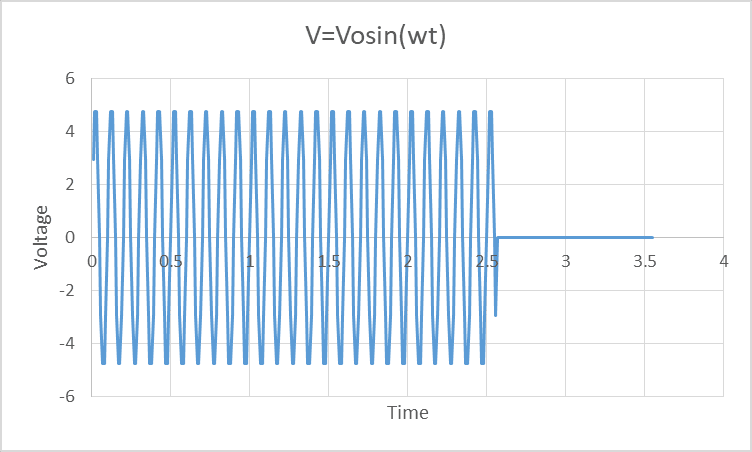
Figure 1, A pulsed radar signal is shown above. This is a single unchanging frequency over the time interval shown.

The FFT of the signal in Figure 1 is represented in Figure 2. The curve of magnitude versus frequency has a fairly tight spectral peak that drops to near zero on each side of the peak. A common adaptation to this curve is to plot the values as 10*log10 (Magnitude). This allows weak and strong signatures to be studied without adjusting scale. Figure 3 is the 10*log10 of Figure 2.

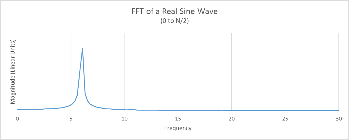
Figure 2. This is the 256-point FFT output of the radar signal shown in Figure 1. The subtitle of this plot and all other FFT plots in the tutorial refer to the use of only 0 to N/2 output frequencies. The N/2 to N points are artifacts of the FFT that should be ignored when performing real FFTs. When applying complex FFT’s, the full FFT spectrum is used.

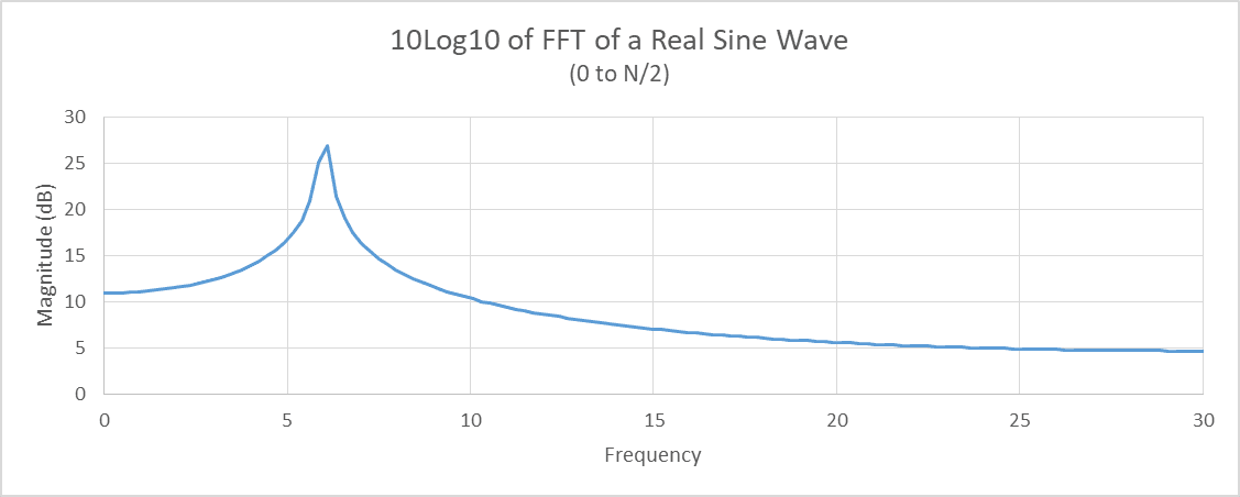
Figure 3. This is the 10*Log10(Figure 2).

Another common tool used in FFT analysis is to increase the number of points in the FFT to gain resolution. Figures 2 and 3 are computed using a 256-point FFT, so going to a 512-point FFT will increase spectral resolution. One may ask, how can we execute a 512-point FFT when we have only 256 samples of data? The answer is padding, which is the addition of zeros to the existing data sample set. In this case, 256 zeros will be added to the 256 of real data points. This is one of the many wonderful benefits of using the FFT. Adding zeros does not have any negative effect – it only permits higher frequency resolution. If this was a pulse Doppler radar, the padding of the FFT will result in finer Doppler resolution. Figure 4 is the 512-point FFT using the 256 points of signal in Figure 1 plus 256 points of zeros as input. Figure 5 is the 10Log10 of Figure 5.

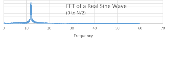
Figure 4. This is the 512-point FFT of the signal in Figure 1 which has been padded with 256 zeros.

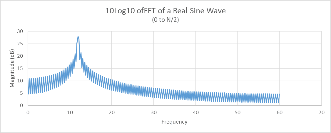
Figure 5. This is the 10*Log10(Figure 4).

Now let us apply one of the windows mentioned earlier – the Hann window. The Hann window is perhaps the most popular window function in pulse-Doppler processing. The Hann window is defined as:

w(k) = 0.5[1-Cos(2πk/N)] ,

where k = the wavenumber = 2π/wavelength

             N = number of points in the FFT, or

             ½ * number of points in the FFT if padded.

The Hann window function for 512 points is plotted in Figure 6. To apply the window function, we multiply the function noting to recalculate it for 256 points to the signal in Figure 1. Figure 7 is the plot of Figure 1 with the Hann Window applied.

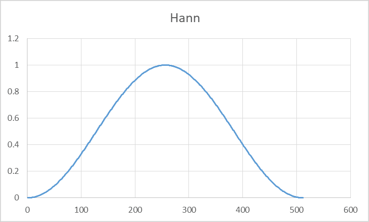
Figure 6. This is the Hann ( Hanning ) window function.

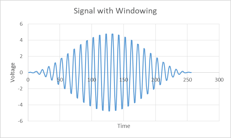
Figure 7. This is the signal in Figure 1 with the Hann window (Figure 6) applied.

Once the windowing function is multiplied and extra zeros are added to the signal, we can compute the 512-point FFT of the signal in Figure 7. Then take the 10Log10 of the FFT results and we end up with Figure 8. There are two changes in Figure 8 that are immediately noticeable from Figure 5:

The curve tappers away faster from the peak frequency in Figure 8 (note the y-axis intercept is less than -20 in Figure 8, whereas it is just below -10 for Figure 5). 
The main lobe (the width of the peak frequency) is wider in Figure 8.

Point number 2 is a fundamental condition of the main lobe of any signal that has had a window function applied – it will get wider. Figure 9 is a comparison of Figure 8 and Figure 5 on the same graph. Figure 10 is a zoom of Figure 9. Note that we can also add another difference in the two curves – the windowed FFT has a lower peak signal strength. So now one may ask, why would I want to apply a function to my data that lowers my peak signal strength and broadens my main lobe?

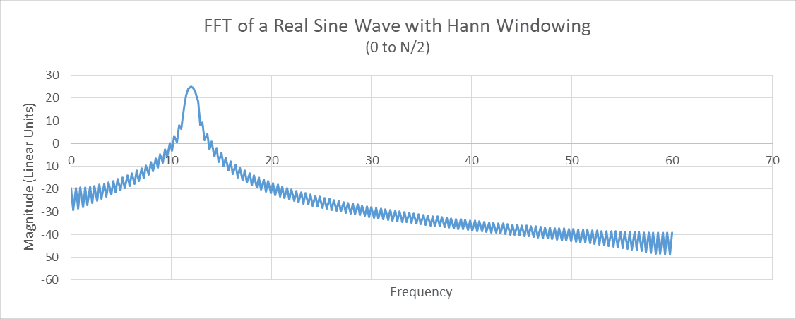
Figure 8. The 10Log10 of the padded 512-point FFT of the signal in Figure 7.

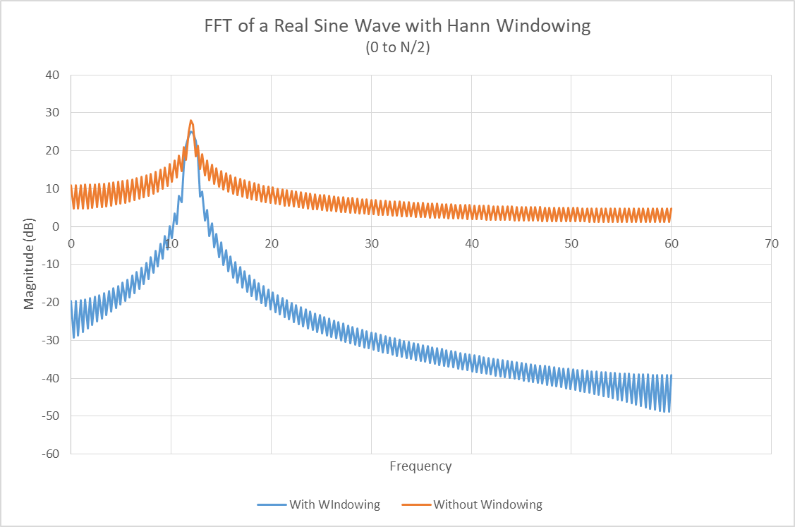
Figure 9. The comparison of the FFT of the signal in Figure 1 with and without windowing

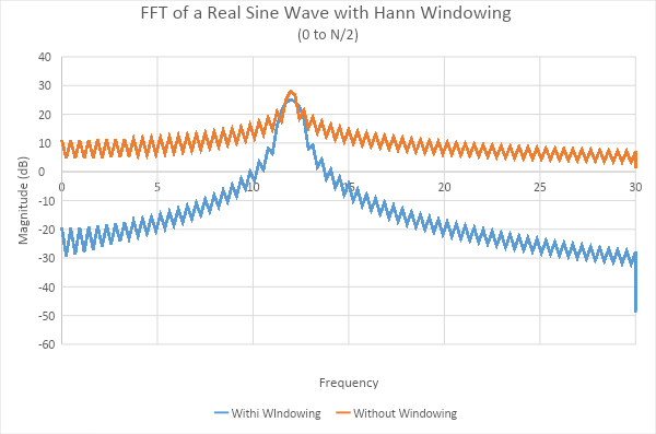
Figure 10. A zoom of Figure 9.

The answer to the question (why use a window) is to reduce spectral leakage. By applying the windowing function, two or more objects can be resolved in frequency that may not have been without windowing. In addition, weaker signals will be detected even when close to strong reflected signals. As an example, a VW Bug will be seen next to a large cargo truck. So in other words, there is higher signal-to-noise for most objects when a window is applied.

As an example of improved improvements, please look at Figure 11. It looks like Figure 1, but in closer examination one may notice that the peak voltage in Figure 11 is not as uniform at the top and bottom of the waveform as compared to that in Figure 1. The signal in Figure 11 consists of two separate signals. One signal is the same as in Figure 1: A*sin (2π*f*t), where A = signal amplitude, f= frequency and t = time. The second signal is 100 times smaller (-20dB) than the other signal and its frequency is 25% higher.

Let us take the padded 512-point FFT of the signals in Figure 11 – this yields Figure 12. This FFT has no windowing function applied. Now look at Figure 13 to see what windowing adds. Hann windowing is applied to the signals in Figure 11. The two signals are clearly visible. Figure 14 is a comparison of Figures 12 (no windowing) and Figure 13 (Hann windowing). Figure 15 is a zoomed-in version of Figure 14.

Figure 11. Two signals combine in this plot. The difference is barely noticeable from Figure 1. One signal is 100 times larger than the other, and one is 25% higher frequency.

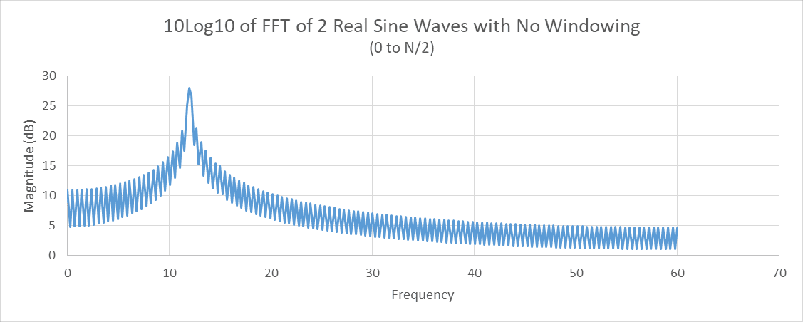
Figure 12. This is the padded 512-point FFT of the signals in Figure 11. There has been no windowing function applied here.

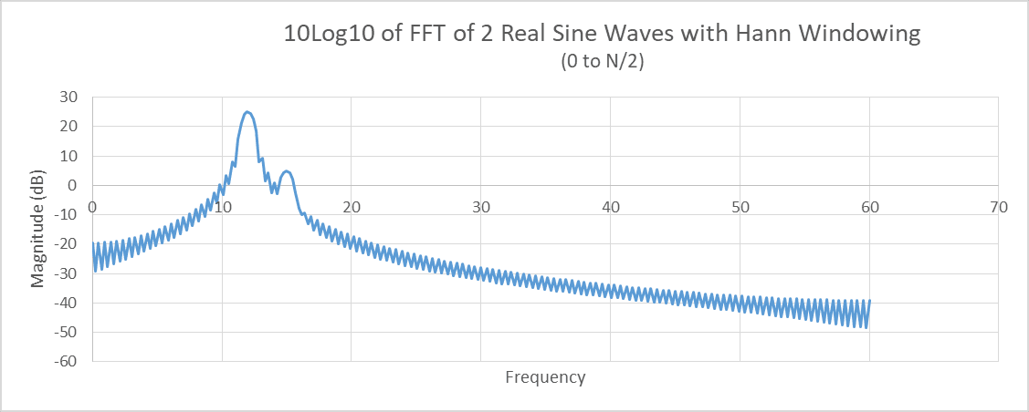
Figure 13. This is the padded 512-point FFT of the signals in Figure 11 with windowing. The second signal arises from the noise Note that the 20 dB difference in peak signals matches the analog signal strength difference mentioned earlier in this text.

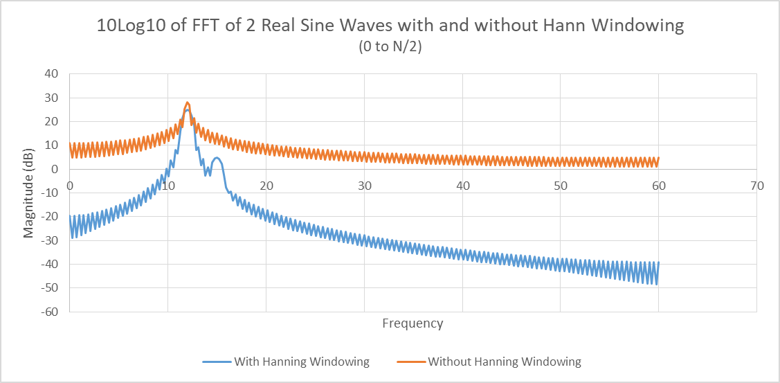
Figure 14. This is a comparison of Figures 12 (without windowing) and Figure 13 (with windowing).

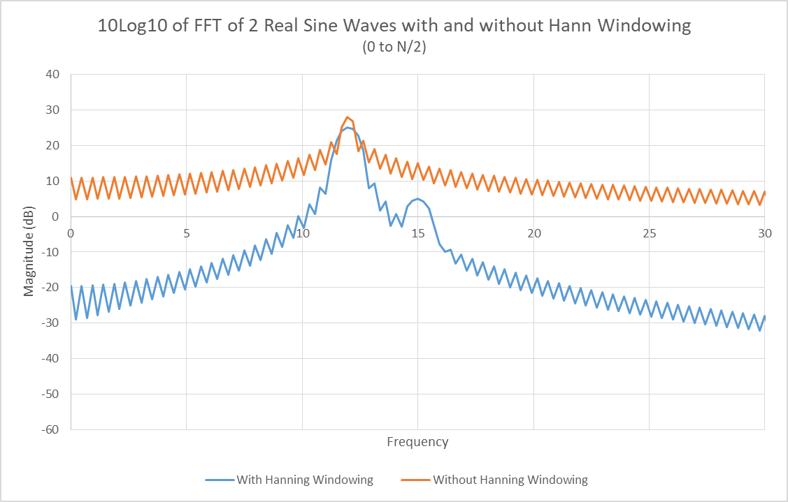
Figure 15. This is a zoom in on Figure 14.

Hann windowing is very effective in improving signal-to-noise and reducing spectral leakage. Depending on the focus of the signal processing, other windows may be better suited. Let us consider the Hamming window. What is the difference between Hamming window and Hann window functions? See Figure 16 – this is a comparison of the two window functions. Note that the Hamming window does not go to zero at the tails. Figure 17 shows what the two window functions do to the same 2 signals found in Figure 11.

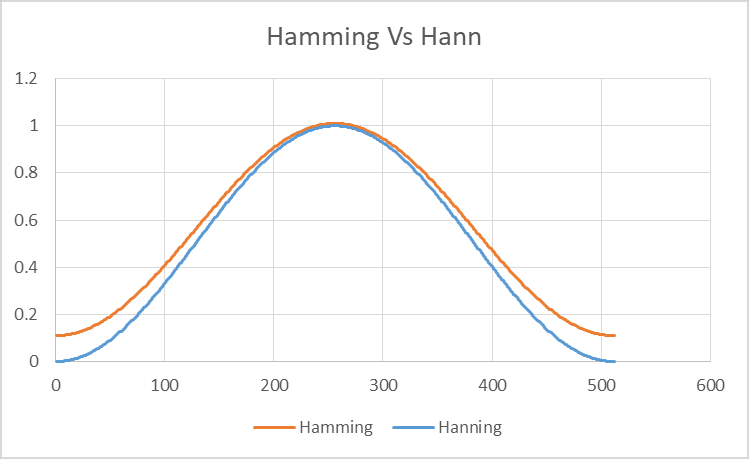
Figure 16. The Hamming and Hann window functions are shown above.

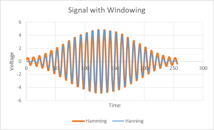
Figure 17. This is the resultant signal when Hamming and Hann window functions are supplied to the signals in Figure 11.

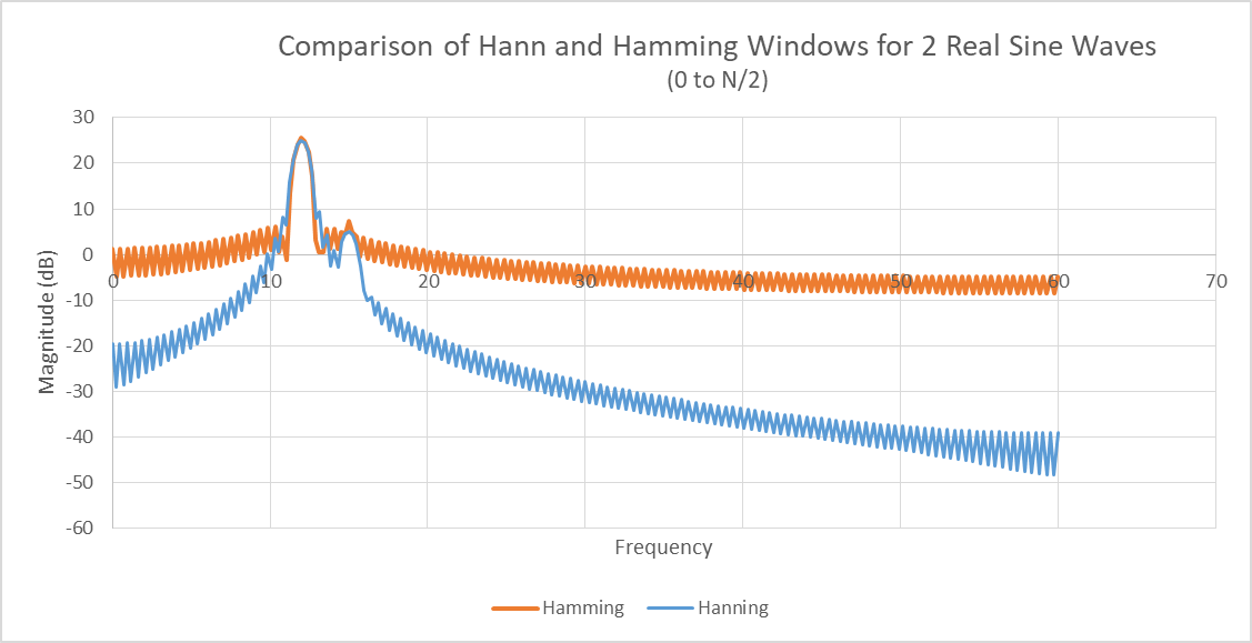
Figure 18. The Hamming and Hann Windows are applied to the signals in Figure 11, and a 512-point FFT is taken on the signals. Note that the Hann is far better at raising signals from the noise, but the Hamming window offers lower first sidelobes, a slightly higher peak, and a slightly narrower main lobe response. Hann windowing is by far the more popular of the two windows for Doppler processing..

Antennas

The typical radar antenna beam has a sin(x)/x pattern that looks like the plots in Figure 19. This pattern forms because the antenna dimensions are finite. If the antenna were the size of the Earth, the pattern would be like a laser beam. The mainlobe is at the center of the plot, and is in the direction the antenna is pointing. The minor lobes that are to the left and right of the mainlobe are the sidelobes. Note that the largest sidelobe level of a uniformly illuminated antenna is about 13 dB lower than the mainlobe level. Unfortunately, this can become problematic when it comes to detection.

The radar cross section (RCS) is the measure of the size of an object to radar. A human is normally 0.5 to 1 square meter (0 dBsm) A car can be 10 to 20 times larger (15 dBsm) than a human, and a school bus comes in at over 100 times larger than a human (20+ dBsm) . If a human were walking through the mainlobe of the radar, and a car and bus are in the sidelobes, their effective signal-to-noise ratios may be the same. See Figure 20. If a bus were detected at a distant sidelobe, the radar could determine that the object detected was a human in the mainlobe because the measured RCS is equivalent to a human. And the fact that the detection of the bus was at an angle far away from the mainlobe, the position of the object on a map would be erred by this angular error in detection.

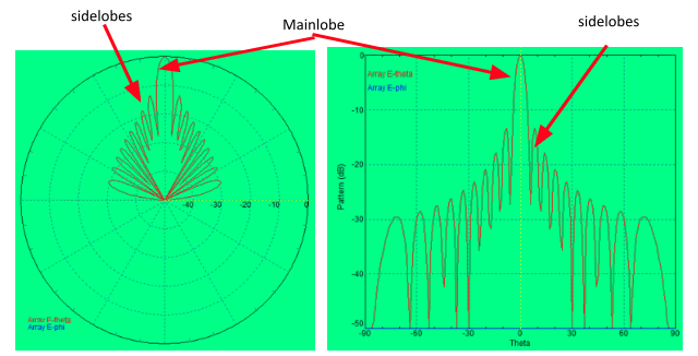Figure 19. This is the antenna pattern of a linear array antenna of 10 linear elements spaced 1/2 wavelength apart for an X-Band radar. This antenna has no windowing (weighting) of the power distribution to the radiating elements. The LEFT plot is the polar plot representation of the antenna pattern. The RIGHT plot is the antenna pattern in Cartesian coordinates.

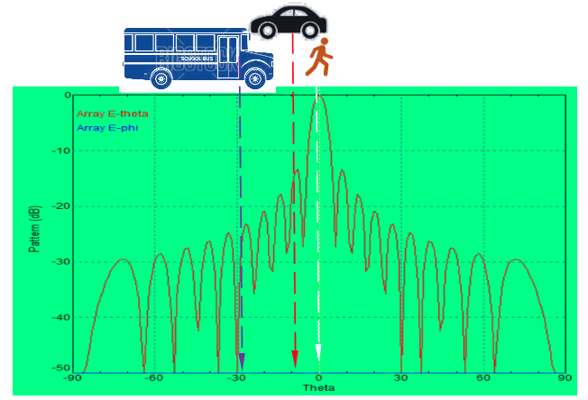Figure 20. The plot is the sin(x)/x pattern of an antenna. Assuming the cartoon characters are located at large angles from the center of the antenna beam, these detected objects would appear to be human-sized. For instance, the bus may have an RCS of 30 dBsm, but it appears at 26 degrees from boresight. The larger RCS plus pulse integration are offset by the sidelobe level, so the radar will incorrectly assume it is a person. 

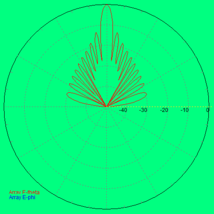
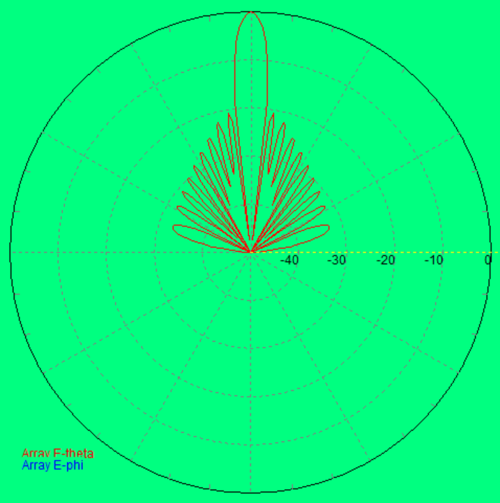
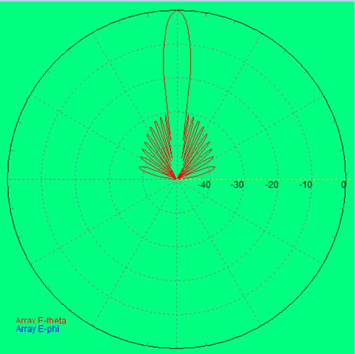
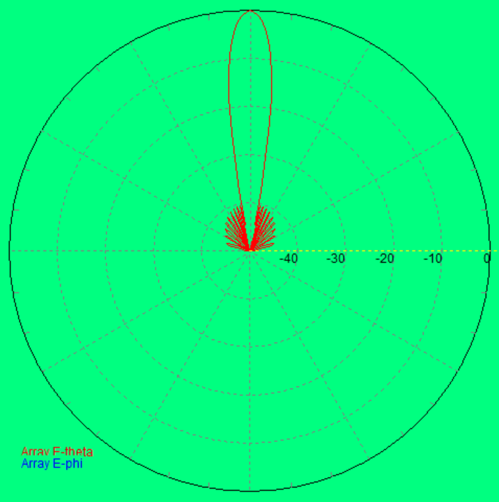
To combat the issue of high sidelobes, a window can be applied. (Note: the more common expression to use is antenna weighting rather than windowing.) By far the most popular antenna sidelobe reduction function is the Taylor window. It is also one of the more complicated windows requiring polynomial coefficients to be computed. The two main parameters of the Taylor window are the sidelobe level (e.g., -30 dB), and n (also known as n-bar). The parameter n is normally set between 1 and 6. Figure 21 shows 4 antenna patterns. Figure 21a is uniformly illuminated (no window), 21b has a Taylor window with -20dB sidelobes and n=2, 21c is a window function of -30 and n=0, and 21d is -40 and n=6.

(a)                                                (b)

(c)                                               (d)

Figure 21.(a) is a uniformly fed (no windowing) antenna pattern. (b) is a pattern with Taylor weighting of -20 and n=2, (c) has Taylor weighting of -30 and n=4, and (d) has Taylor weighting of -40 and n=6.

Table 1. The antenna values of a 10 GHz radar with and without windowing (weighting).

Looking at Figure 21, it is clear that the sidelobe reduction granted by the Taylor window function would greatly reduce the occurrence of positional pointing errors.

Glossary (Terms used in the text):

Pulse: The short burst of RF energy transmitted by many types of ranging radars. RF switches are triggered to produce these pulses of energy by rapidly interrupting (like a light switch) the output of a continuous wave source (like an oscillator).

Pulse Repetition Frequency (PRF): The rate at which pulses are transmitted in a radar per second.

Doppler: The change of frequency caused by motion from an object. The emitted frequency from a radar transmitter is shifted upwardly if the object is moving toward the radar, and downwardly if the object is moving away from the radar.

Doppler Resolution: This is the smallest increment of speed that the pulse- Doppler radar can detect. A radar that is trying to detect people movement will have Doppler resolutions of a few centimeters/second.

FFT Plot (Range-Doppler Plot): The FFT is used to convert radar time domain data to frequency domain. Detected objects and their Doppler signature are plotted in an FFT Plot. The x-axis represents the Doppler Frequency (which can be converted to Doppler Speed), and the y-axis is range. The Range-Doppler Plot is also referred to as the Doppler Time Intensity Plot, especially if it is recorded as a data stream.

Padding: Adding zeros at the end of a valid input dataset for an FFT. If 256 points are captured by the radar’s analog-to-digital board, then another 256 zeros would be added at the end. The output of the FFT will be at a finer resolution than without the zeros. The negative effect of padding is the increase of computing power required for the FFTs. 

Magnitude: This is the signal strength. In the plots of this paper, the units were not specified, but are commonly supplied in voltage or in power.

RCS (Radar Cross Section): This is essentially the size of an object as seen by a radar. Its value is a function of the object size, its dielectric properties, and orientation.