


In this article we shall perform the anatomy of a simple but efficient convolutional network (CNN), the LeNet-1 neural network.
History of the LeNet-1 neural network
The LeNet architecture came historically as an attempt to classify 2D images and to produce a simple convolutional network that could be more efficient than
- ‘small’ neural networks, which have difficulties learning training sets, and
- large neural networks which contains much too parameters to be conveniently exploited.
It is possible to design very specific neural network architectures, which are dedicated to recognize 2D maps, while these networks are eliminating noise, distortions and fluctuations inside the input data.
Such specific networks are called convolutional networks.
Convolutional networks can be designed to exploit ‘local’ patterns and combine the individual results into a whole. This is the idea of the LeNet architecture.
The LeNet architecture was introduced around 20 years ago by Yann LeCun and other researchers and an initial description of the network design can be found in [1] .
Overview of LeNet-1
LeNet-1 ( and other following LeNet & CNN architectures ) are based on two main ideas acting as the pillars of such models:
- Building a set A of local area A in the 2D map unique common weights, which can be called units . The output of A are the feature maps, e.g 2D maps which are outputted from areas with a common weight;
- ‘Cascading’ local convolutional feature maps applied to several hidden layers.
In the following, we will detail these designs specifics:
Feature map System
A feature map is created by applying a convolution operation to the initial matrix. Eg:
feature Map = input matrix * kernel matrix
where ‘*’ is the convolution operator. This means that, in fact, only a few weights will be used, the ones inside the kernel matrix.
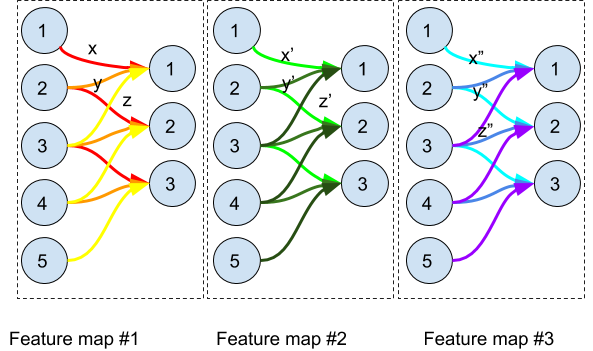
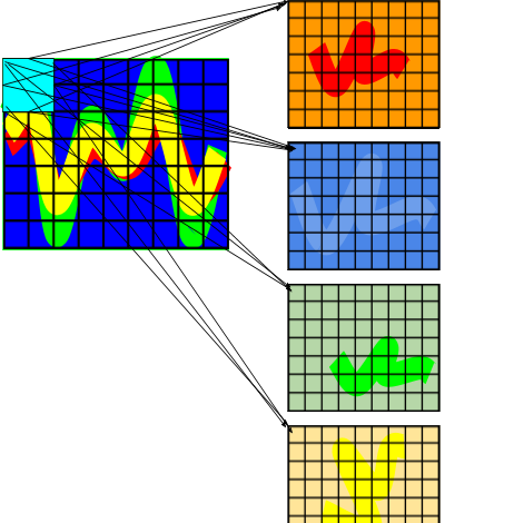
In the above illustration, we demonstrate the concept of common group of weights. A feature map is created by convolution of a plan with a kernel/filter. The feature map #1 is created by the kernel (x,y,z) in the following way:
b1 =`sigma`(x*a1+y*a2+z*a3)
b2 = `sigma`(x*a2+y*a3+z*a4)
b3 = `sigma`(x*a3+y*a4+z*a5)
etc...
Where (ai)1`<=`i`<=`5 are the (five first) neurons of the N hidden layer, (bi)1`<=`i`<=`3 the (three first) neurons of its successor, the (N+1) hidden layer and is an activation function.
All the same, the feature maps #2 and #3 are created respectively by the kernels (x',y',z') and (x",y",z").
b1 =`sigma`(x'*a1+y'*a2+z'*a3)
b2 = `sigma`(x'*a2+y'*a3+z'*a4)
b3 = `sigma`(x'*a3+y'*a4+z'*a5)
b1 =`sigma`(x''*a1+y''*a2+z''*a3)
b2 = `sigma`(x''*a2+y''*a3+z''*a4)
b3 = `sigma`(x''*a3+y''*a4+z''*a5)
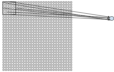
Local connectivity
The reasons for considering local connectivity comes from the fact that it may seem inordinate to use networks with fully-connected layers in order to classify 2D maps (‘images’). Indeed, such a network architecture does not fully address the spatial nature of the data. A fully connected network would consider all the same input pixels which are close to each other or to the contrary who are far from each other.
So LeNet-1 (and in fact any typical CNN) does not connect every input pixel to every hidden neuron. Connections are done only in small localized region of the image.Such localized region are defined by a Local receptive field, a submatrix of relatively small dimensions, which is in fact the convolution kernel.
LeNet-1 Detailed Design
LeNet-1 applies originally to 16x16 pixels maps which are extended to 28x28 pixels maps by adding a 6 pixels blank frame around the original map so to avoid edge effects in the convolution computations.
In the original LeNet-1 architecture, the input is therefore a 28x28 pixel image data. This represents 784 input neurons (+ the bias neuron). It doesn’t matter how they are ordered. We assume here that they are ordered by lexicographical order on the pixels coordinates pij, e.g., pij < pkl if i<k or (i=k and j<l).
The whole set of possible values of the input is already huge, e.g., it is 2784 `~~` 10236 which means that it is impossible to consider an exhaustive list of all the values.
Over that initial plan, 4 regions - aka feature maps - from four 5x5 kernels will be created.
Description of the First layer
The first layer (the input isn’t considered to be a layer) will therefore have 4 feature maps of size 24x24 each, which makes 4x24x24=2304 neurons (+1 bias neuron)
We represent here the input neurons ordered as a matrix:
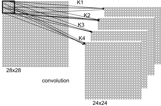
Over that initial input matrix, 4 filters K1,K2,K3,K4 of the size 5x5 ( e.g 25 weights each ) are applied by convolution so that they generate 4 feature maps of size each 24x24.
The size C of a convoluted feature map is given by the formula:
C=(I+2P-K)/S+1
Where I is the size of the input matrix, P the margin, K the size of the kernel and S the stride.
Here C=(16+2*6-5)/1+1=24.
The values of the first layer are given by the convolution formula:
b(s)i,j = `sigma (b+sum_(l=0)^4 sum_(m=0)^4` K(s)l,m* aj+l,k+m )
Where b(s)i,j is the (i,j)th neuron , lexicographically counted, of the s-th feature map, K(s)l,m is the (l,m)th neuron , lexicographically counted, of the s-th 5x5 filter and aj+l,k+m is the (j+l,k+m)^th neuron , lexicographically counted of the input and b is the bias neuron. is an activation function , usually the sigmoid.
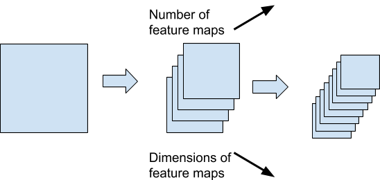
The design consists in refining more and more possible patterns into a bigger set of feature maps which are in turn of smaller and smaller sizes.
All layers

LeNet-1 has an overall of 3 convolutional layers C1, C2, C3 and 2 pooler (sub-samplers) layers S1, S2. The network can be described by the following flow:
INPUT `rightarrow` C1 `rightarrow` S1 `rightarrow` C2 `rightarrow` S2 `rightarrow` C3 `rightarrow` OUTPUT
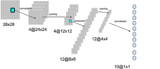
Once the input has been convoluted into 4 feature maps, each feature map is pooled into 4 corresponding feature maps of dimensions 12x12 each. The pooling is done over sub-matrices of dimension 2x2 so that it divides the amount of neurons by 2*2 , eg 576 neurons + the bias neuron. In the next layer, convolution is done again this time with a 3 filters of dimensions 5x5 each. Since the convolution is done on each of the 4 pooled feature maps, this multiply the amount of feature maps to 4*3=12 but the dimensions of each new feature map is reduced from 12 to C’=(12-5)/1+1=8. This creates 768 neurons (+ bias). This new layer is pooled again so the size is reduced to 192 neurons (+ bias) . Finally we perform a final convolution of the 12 ‘tiny’ 4x4 feature maps so to create 10 neurons. (LeNet-1 originally classify handwritten digits from 0 to 9 but the ten categories can be anything else, like a series of airplanes or helicopters, as shown hereafter. We represent the first step of the convolution operation in C1, other steps would refine the patterns and finally would decide of a category. Here for example, we represented the RADAR image of a helicopter.

Comments on the LeNet-1 architecture and its use for RADAR data classification
 The LeNet-1 architecture, which is quite ancient in terms of neural networks, is inspired by the way the brain processes optical information.
The series of convolutions and pooling processes an image so to extract more and more adequate features. The final weights given to these features will determine the classification of the data into one of the possible categories.
LeNet-1 can work very well with RADAR imagery, e.g., RADAR 2D diagrams because the color codes and the patterns can be treated as image recognition, e.g., with the same technique used for recognizing a handwritten digit.
Of course LeNet-1 has improved since the time but in the present article we wished to go into the details of a typical convolution network.

References and Further Reading
- More articles on artificial intelligence (2019 - today), by Martin Rupp, Ulrich Scholten, Dawn Turner and more
- [1] LEARNING ALGORITHMS FOR CLASSIFICATION: A COMPARISON ON HANDWRITTEN DIGIT RECOGNITION (2000), by Yann LeCun, L. D. Jackel & al, AT&T Bell Laboratories