


One of the most powerful statistical estimation techniques, which is widely applied in navigation, radar tracking, satellite orbit determination, autonomous driving, and many other fields is the Kalman filter. This digital filter provides a quite accurate estimation of the next state (position, movement, temperature, etc.) from any possible noisy input signal, in real time, which makes it very suitable for radar navigation and tracking purposes.
For the tracking feature in ATC II, we make use of the Kalman filter principle, to estimate the detected moving targets. In the following figure, the block diagram of the tracking feature is shown.
![]()
Figure 1 Block diagram of tracking feature
The tracking feature of ATC II consist of four steps:
- Signal detection – DET
- Phase Shift detector – PH - DET
- Association – ASO
- Kalman filter – KF
1. Signal Detection
The signal detection step has already been explained in the context of MTI and MTD (see ATC I and ATC II to look at their composing blocks). Also in the context of tracking as treated in this article, is servces as a signal pre-processing step, to filter out the trivial clutter information.
2. Phase Shift Detection
The second signal pre-processing step is the phase shift detector. The main aim of this block is to detect the phase shifts from two consecutive pulses. Two consecutive pulses which have a Doppler-frequency will not have a regular/expected phase shift in comparison with two consecutive pulses of stationary targets. In this way, the first estimation if a target is moving or standing, is done in this step.
However, only detecting the phase shift of two consecutive pulses, does not assure that these reflections are coming exactly from a relevant moving target or maybe moving leaves of a big tree, which appears to be in the field-of-view of the radar. That is the reason, why the association step is employed in this tracking system.
3. Association (ASO)
The ASO step performs a phase gating association of the detected signal peaks and a time association of the coming reflections.
The phase gating does check if the phase shift difference between two consecutive pulses does appear within the expected gates.
If not, then the pulse is filtered out.
If the phase is inside the gating boundaries, then the pulse information is processed to the time association step from where the time counter does check if the signal peak is coming from the same target for at least two cycles.
If yes then the signal is processed to the Kalman filter, if not then the signal is discarded, and the next signal track will be created on the next cycle.
4. Kalman Filter
The final step in the tracking feature is indeed the Kalman filter. Since there is no exact information about the velocity of the target, which is detected, the pre-processing steps are more than necessary to prepare the signal for Kalman filtering.
The following figure does show the steps within the Kalman filter itself.
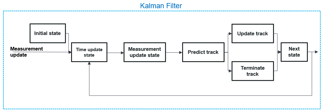
Figure 2 Block diagram of tracking feature
First the initial states of the system are determined, in this case the position variable x and the prediction step S at the state i=0:
X0 = 0 and S0 = 0 (1)
Afterwards, the time update states are determined as following:

(2)
In the measurement update state, the noisy inputs are considered, and the target position is predicted. First the Kalman gain Gi, and prediction step Si are defined for the ith state:
 (3)
(3)
where ß does represent the standard deviation of the radar device.
Finally, the measurement update is performed as following:
 (4)
(4)
where the yi is the noisy input signal.
After the track is predicted then the output track is updated using the nearest neighbour method between two consecutive tracks, to determine if the track is within distance gating boundaries.
If this track is estimated within the range gates the track for the output signal is updated, and the time update states are redetermined for ith+1 state as defined in equation (2) via the recursive path as stated also on Figure 2.
If the predicted position cannot be associated with the nearest neighbour method, then the respective track is terminated. And like this the filter iterates to the next state.
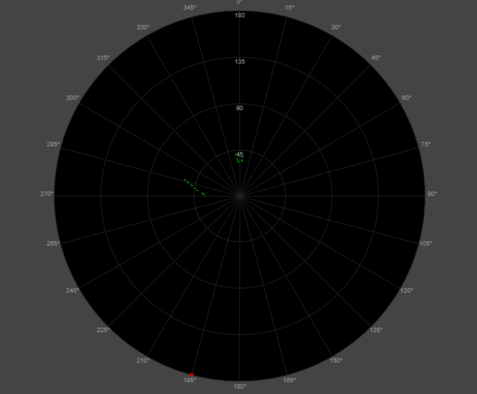
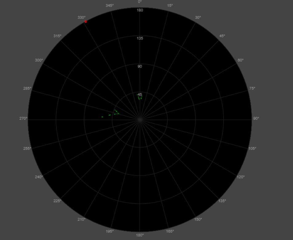
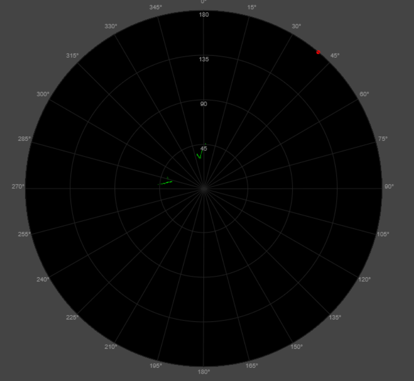
In the following figures some of the estimated Kalman filter tracks are shown in PPI scope.
The Kalman filter is part of the ATC II package. ATC II is a module within the FreeScopes Digital Signal Processing Environment for Radar Signals, which includes a whole set of advanced filters. ATC II also includes a set of "atomic" blocks like Zero Velocity filter, Clutter Map, or a Signal Delay Block, which enables students, trainees and researchers to compose their composite (advanced) filters.
Talk to us to discuss how to use FreeScopes and SkyRadar's training radars in your institute.