


In the present tutorial, we shall explain what are the Support Vector Machines (SVMs) and how the kernel-based SVM classifiers are working.

SVMs are an important class of Machine learning algorithms and they have been used in a successful amount of projects for RADAR objects automatic recognition. In what follows we seek to introduce the main basis for the reader.
Support Vector Machines operates as classifiers using several properties of linear algebra. They can separate a dataset into higher-dimensional spaces using kernel methods.
They require some understanding of basic functional analysis and linear algebra and so their theoretical background have not always made them the choice for concrete classificator implementations. This said, they often achieve similar or even better results than the equivalent neural networks classifiers or the probability-based classifiers.
Some Quick Facts About SVMs
SVMs are a special class of Machine learning models named “nonparametric” models. “Nonparametric” means that the parameters only (and directly) depend on the training set.
The only information given to a SVM in a supervised training is to learn from a set of couples `(x^i,C^i)` where `x^i` is a n-dimensional vector and `C^i` is a class label, among k possible classes labels.
SVMs will seek to build decision functions to classify the data. For this, they will only rely on a special set of data , from the training set, namely the support vectors. This means that an important amount of the training data won’t be used at all.
SVMs belong to a family of generalized linear classifiers and they can be seen as an extension of the perceptron.
Some Linear Background
SVMs are using decision functions to separate several sets of data.
In the simplest case, linear binary classification, we consider a set which must be separated into two subsets `B` and `C`.
The set `A` is here a set of vectors `x=(x_1,...,x_n)` in a n-dimensional space.
The separation is done via a function such that `g(x)>0` for all x such that `x in B` and `g(x)<0` for all x such that `x in C`. The subspace `H` defined by `{x,g(x)=0}` is the border between the two sets.
Finding a function `g` is of course always possible since it is enough to define it over the sets `B` and `C`.Of course we look for special, generic, type of functions.
The most simple function is a linear function:
`g(x)=w^_|_x+b` where `w` is a constant vector and b a numerical bias. This can also be written:
`g(x)= sum_(i=n)^(i=1)w_ix_i+b`
It is not always possible to find such a function . If it is possible
and
are said to be linearly separable.
From this it is possible to achieve multi-class seperation. There are several ways to define multi-class separation, it can be achieved by ‘all-in’one’, binary tree or pairwise separation, for instance.
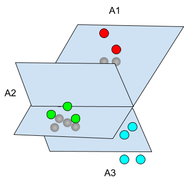
For example, it is possible to consider that, in the case of `N` classes `A_1, ..., A_N`, we define `N` separation functions `g_1, ..., g_N` and we claim that x belongs to an `A_i` if `g_i(x)>0` and `g_i(x)<0,j!=i`.
Geometrically speaking, this can be easily visualized as the building of geographical areas from hyperplanes. In the example above, we seperated 3 areas `A_1, A_2, A_3` by using 2 functions `g_1, g_2` such that the signs of both `g_1(x)` and `g_2(x)` decide if x belongs to `A_1`, `A_2` or `A_3` .
Hard Margin concept
The hard Margin M is defined for two linearly separable sets B and C.
If we can find a linear function such that `g(x)=w^_|_x+b` and:
`g(x)<=-1<=>x in B`
`g(x)>=+1<=>x in B`
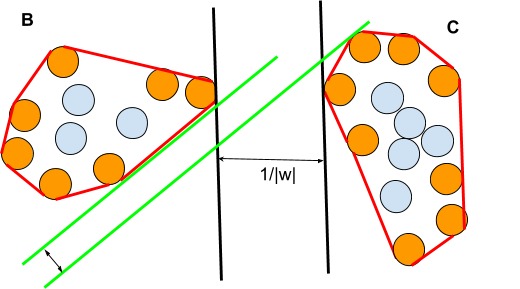
The distance between the two hyperplanes is 2d with `d=1/abs(w)`, this is the (hard) margin.
If we label the N vectors of `B bigcup C` by `(x^j,y^j)` and `y^j=+1<=>x^j in C`, `y^j=-1<=>x^j in B` then we seek to find a hyperplane defined by `w` such that the following optimization problem is solved:
`MAX_w1/abs(w),y^j(w_|_x^j+b)>=1,j=1...N`
That optimization problem is the hard-margin problem for the support vector machines.
The motivation for maximization of the margin is because it will provide the most ‘generic’ classification when considering further samples, not from the training set.
Definition of Support Vector
To visualize it, one must introduce the notion of support vectors. These are the vectors belonging to the border of the convex hull of each set. (I)
A convex hull is the smallest convex set containing a given set.
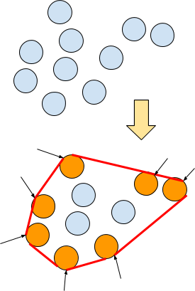
In the above picture we pictured the convex hull in red and the support vectors in orange. There are 7 support vectors among the 10 vectors. Only these support vectors will be used for the computation of the separating hyperplane.
Note that it is also possible to transform B or C via a translation and /or rotation (affine transformation) for instance, eg to apply a linear transformation defined by a unit matrix `Z` such that `C'=ZC`. Still only the support vectors - as we defined them - will be to consider.
Some definitions(II) of support vectors may differ, e.g. only including a subset of the border of the convex hull consisting of all the vectors having contact points with at least one separating hyperplane (see fig below).
In such definition (II) the support vectors are defined for pairs of sets.
Optimization problem (Linear case)
In case the set are linearly separable, we have to solve the following optimization problem:
Given N vectors `x^1,...,x^n` of a set A and their associated classes `y^1,...,y^n in {-1, +1}`
Find vector(s) `w = (w_1, ..., w_n)` such that we have
`MAX_w1/abs(w)`
with the constraints `y^j(w^_|_x^j+b)>=1,j=1...N`
Since `abs(w) = sqrt(w_(1^2) + ... + w_(n^2))` , this is a quadratic optimization problem.
This problem is not very hard to solve.
We can use a classical Lagrangian optimization technique. Here we will consider the (dual) equivalent optimization problem:
`Q(w,b,lambda_1,...,lambda_N)=1/2w^_|_w-sum_(i=1)^Nlambda_i(y^j(w^_|_x^j+b)-1)`
`MAX_lambdaMIN_wQ(w,b,lambda_1,...,lambda_N)`+Kuhn-Tucker Conditions
`lambda>=0`
This is equivalent to:
`MAX_(lambda>=0)Q(lambda)=sum_(i=1)^Nlambda_i-1/2sum_(i,j=1)^Nlambda_ilambda_j(x^i)^_|_x^j`
The Lagrangian parameters `lambda_1, ..., lambda_N` if they exist, define w and b.
`w=sum_(i=1)^Nlambda_i y^ix^i`
`b=y^i-w^_|_x_i=1/abs(A)sum_(i=1)^(i=N)(y^i-w^_|_x_i)`
Such SVMs are named the Hard-Margin SVMs.
Soft Margin
If the data are not linearly separable, e.g the convex hulls of the sets to seperate are not disjoint, then another technique must be seeked, this is named the soft-margin technique.
In the non-linearly separable case, there are two subcases.
We need to introduce special variables `z^j>=0`, named slack variables and defined such that:
`y^j(w^_|_x^j+b)>=1-z^j`
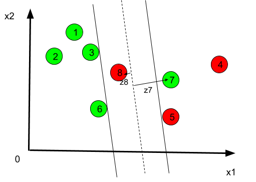
In the previous example, we have `z^((7))>1` and `z^((8))<1`.
When we correct with the stack variables:
- If a slack variable is <1 , then the corresponding data is still correctly classified (even if the margin is not optimal in such case) (case I)
- If a slack variable is >1 then the corresponding data is not correctly classified (case II).
We need therefore to find the optimal hyperplane with the minimal amount with slack variables are minimal. For this we introduce a very important parameter, named the C-parameter and we have the soft-margin optimization problem:
`MIN_w1/2abs(w)^2+Csum_(i=1)^N(z^((i)))^p`
with the constraints `y^j(w^_|_x^j+b)>=1-z^((j)),j=1 ... N`
The solution of this problem are the soft-margin hyperplanes.
The values of p are typically chosen to be 1 or 2 and depending on the choice, the soft-margin hyperplane is called respectively L-1 or L-2 hyperplane.
The resolution of the optimization problem is essentially the same as with the hard-margin, using Lagrangian multiplicators.
Mapping to higher-Dimensional Space
The soft-Margin SVM may not always be suitable because it includes some mis-classified points (‘noise’) and one may want to look for a classification method without such problems.
If the two sets `B` and `C` can be separated by a nonlinear function `varphi` e.g such that `varphi(x)`is positive on `B` and negative on `C`, then one may try to find a mapping between the n-vector space where the classifications hold and another vector space, which can be of infinite (enumerable) dimension.
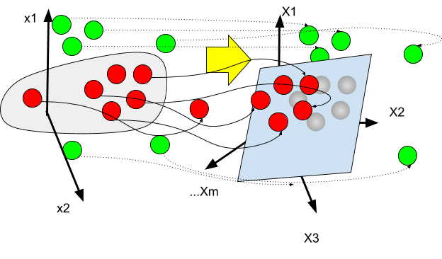
The original finite-dimensional space is mapped into a higher-dimensional space - the ‘feature’ space- , with the goal to make the separation easier in that space.
If we can decompose `varphi` in a sum of ‘elementary’ terms `f_z` such that `varphi(x)=sum_(z)a_zf_z(x_(i_z))`, then we define a mapping F `(x_1, ..., x_n) rightarrowprod_zf_z(x_(i_z))` from the n-dimensional space to a new space `varepsilon`
And claim that the linear function `g(x)=sum_za_zX_z` over `varepsilon` separates the set B and C.
For example, if we consider `varphi(x)=x_1^2+4log(x_1)+x_2^3` in a 2-dimensional space. We can map it to a 3-dimensional space `varepsilon` defined by `x->X` or:
\( \left( x_{1},x_{2} \right) \rightarrow \left( x_{1}^{2},log \left( x_{1} \right) ,x_{2}^{3} \right) \)
We can therefore write that `varphi(x)>0rArrg(x)>0` and `varphi(x)<0rArrg(x)<0`where `g(X)=X_1+4X_2+X_3`.
In the above illustration, we represent the mapping from the initial space to the feature space.
In such cases we revert to the hard-margin scenario.
The Optimization problem is :
`MAX_(lambda>=0)Q(lambda)=sum_(i=1)^Nlambda_i-1/2sum_(i,j=1)^Nlambda_ilambda_j(x^i)^_|_x^j`
Computation of the products `(X^i)^_|_X^j` may be very difficult.
For example in the example we mentioned previously, we would have:
\( \sum _{i,j=1}^{N} \lambda _{i} \lambda _{j} ( X^{i} ) ^{\bot}X^{j}= \sum _{i,j=1}^{N} \lambda _{i} \lambda _{j} ( ( x^{ ( i ) }_{1} ) ^{2},log ( x^{ ( i ) }_{1} ) , ( x^{ ( i ) }_{2} ) ^{3} ) ^{\bot} ( (x^{ ( j )}_{1})^{2},log ( x^{ ( j ) }_{1} ) , ( x^{ ( j ) }_{2} ) ^{3} ) \)
\( =\sum _{i,j=1}^{N} \lambda _{i} \lambda _{j} ( ( x^{ ( i ) }_{1}) ^{2} ( x^{ ( j ) }_{1} ) ^{2}+log ( x^{ ( i ) }_{1} ) log ( x^{ ( j ) }_{1} ) + ( x^{ ( i ) }_{2} ) ^{3} ( x^{ ( j ) }_{2} ) ^{3} ) \)
Kernel-based SVMs
We seek therefore to find a symmetric function `H:(x,y)->H(x,y)` named a kernel and such that `H(x_i,x_j)=X_iX_j`
Introducing the kernel means there is no need to process the (often complicated) feature space directly (Kernel’s trick).
In such a case the optimization problem can be solved because if the kernel is a semidefinite positive function as well, we need to solve a concave quadratic programming problem.
Kernel-based SVMS are a special part of the Kernel classifiers and should be explained in another article.
Conclusion
SVMs to the difference of other classifiers such as the Neural networks need a slightly more important theoretical background. They are not always simple to use in the general case but they may be a very powerful tool with results which can even be better than the equivalent Neural Networks or Bayesian methods.
We invite the reader to consult the references in Annex to get more insight about the concrete implementations of SVM classifiers for the RADAR technology.

REFERENCES
[1] Radar target classification using Support Vector Machines and Mel Frequency Cepstral Coefficients
SEBASTIAN EDMAN
[2] Radar target classification based on support vector machines and High Resolution Range Profiles
S. Kent ; N. G. Kasapoglu ; M. Kartal
[3] An Approach to Automatic Target Recognition in Radar Images Using SVM Noslen Hernández , José Luis Gil Rodríguez , Jorge A. Martin
[4] Radar target classification using support vector machine and subspace methods
Jia Liu ; Ning Fang ; Yong Jun Xie ; Bao Fa Wang
[5] Support Vector Machines For Synthetic Aperture Radar Automatic Target Recognition
Qun Zhao and Jose C. Principe