


The ID3 - or ID3 (Iterative Dichotomiser 3) - is a supervised classifier based on decision tree learning methodology. The ID3 classifier generates a decision tree from a set of data (the training data) which can be used to classify new data.
General principles
The ID3 classifier is not straightforward to understand. There are a certain amount of key notions that must be defined before. The main concept behind the ID3 classification is Information gain. That information gain is defined roughly as a measure of the benefit of the classifier. To understand what information gain is, we must define the notion of entropy.
Entropy of a set of data
Entropy in Information Theory is linked to mathematical theories such as probabilities and measure theory in general. Here we will define the entropy of a set of symbols as such:
Let us consider an alphabet with a set of n symbols: ` S_{1}\text{,.... ,}S_{n} `
Then we define the entropy E of a word w , that is to say a concatenation of symbols, as such:
` E \left( w \right) =- \sum _{i=1}^{i=n}p_{i} \times log \left( p_{i} \right) `
Where ` p_{i}` is the frequency of the symbol `S_{i}` in the word `w` .
As an immediate remark, we see that a word consisting of the repetition of a unique symbol will have an entropy E=0. On the opposite, a word made of the n symbols , eg `w= S_{1}....S_{n}` will have an entropy `E=- \sum _{i=1}^{n}\frac{1}{n}log(1/n) ` that is to say E=log(n).
Additionally, once can define the entropy of a product of words as the weighted average entropy of each words as follows:
` E \left( w_{1},...,w_{k} \right) =\frac{ \sum _{i=1}^{k}n_{k} \times E \left( w_{k} \right) }{ \sum _{i=1}^{k}n_{k}} ` where `n_{k}` is the number of letters in the word `w_{k}` .
Information Gain
Naively speaking, the information gain is the difference between the entropy of a set of data and another set of data after a given transformation. For instance if F is a transformation from the set of words W into ` \prod W ` Then the Information Gain of the transformation F is defined by:
` IG \left( F \right) \left( w \right) =-E \left( F \left( w \right) \right) +E \left( w \right) `
Usually we seek a positive information gain, e.g. the one that makes the new set with less entropy, e.g ‘more ordered’.
For instance, a very simple transformation (which we will use for ID3) consists in partitioning the word w into subsets.
For instance: we consider a set of 3 symbols: A,B and C.
If we take the word w =(AABCCBB), its entropy is equal to :
` E \left( w \right) =-\frac{1}{7} \left( 2Log \left( 2/7 \right) +3Log \left( 3/7 \right) +2Log \left( 2/7 \right) \right) \approx 1.079 `
Now let us consider the function F which transforms (AABCCBB) into (AA),(BCC),(BB)
The entropy of new product of sets is:
`E \left( F \left( w \right) \right) =\frac{1}{7} \left( 2 \times E \left( \left( A \quad A \right) \right) +3 \times E \left( \left( B \quad C \quad C \right) \right) +2 \times E \left( \left( B\quad B \right) \right) \right) `
The first and the third entropy are null and
` E \left( \left( B \quad C \quad C \right) \right) =-\frac{1}{3} \left( Log \left( 1/3 \right) +2Log \left( 2/3 \right) \right) \approx 0.636 `
This means that ` E \left( F \left( w \right) \right) \approx 3 \times 0.636/7 \approx 0.272 `
The overall entropy is quite small and the Information gain is
` IG \left( F \right) \left( w \right) \approx 1.079-0.272 \approx 0.807 `
The information gain corresponds to a reduction in entropy (Information is opposite to entropy).
Here we transformed the set into relatively very well ordered set (2 sets had minimal entropy=0)
In terms of relative gain, we moved from 1.079 to 0.272 so we gained (a loss of)
`IG=` 74.8%
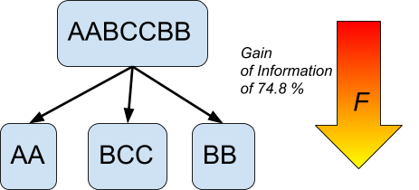
This means that the transformation F, e.g the labeling of the elements, created a gain of information of 74.8%
The next concept we need to define is the decision tree.
Decision Tree
A decision tree is a common structure in decision theory and computer science in general. A decision tree consists of a root nodes (the root of the tree) , internal nodes ( choice nodes), branches (decisions) and leafs (end of the tree)
A decision tree is based on the tree structure, e.g. an undirected graph in which any two vertices are connected by exactly one path, or equivalently a connected acyclic undirected graph.
The process will start at the root node and will go down (or up depending if the tree is represented like the natural trees) through the internal nodes until it reaches a leaf.
The transition from one node to another (or from a node to a leaf ) is done by making a check which can take various forms. In general the process of going down (/up) through the tree consists in defining a set of hypothesis and answering to questions or performing tests to to reach a decision,
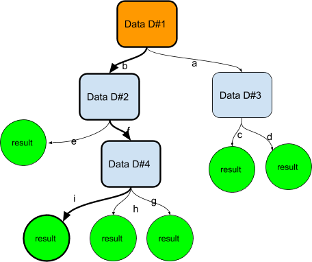
In the above diagram, we represented a root node containing data (D#1) , a test is performed, or an hypothesis is refined among D#1 and this leads to a choice between branches a or b . In that case we consider new data. The test or choice can be a binary one (yes/no) or can be more complex.
In our example, we consider a new set of data, D#2 (which can be totally or partially derived from D#1) and we have to make, again, a choice(/decision) between e and f which involves the data D#2.
We choose f and, again, we must choose between g,h or i , which involves some processing of D#4. This time we choose i and we have reached the bottom(/top) of the tree, e.g a result leaf .
Let us give an example of such a decision tree
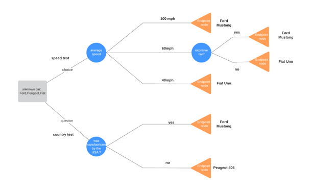
Here we try to identify an unknown car among three possible cars: a Ford Mustang, A Peugeot 405 and a Fiat Uno. For this we go through a decision tree. We can first choose the country test or the speed test and so on, then we decrease the amount of possible cars.
Often Decision trees are based on the probability of realization of certain data or events which can be estimated from statistical samples.
Now that we have the main concepts we can start to detail the principle of the ID3 classifier.
The ID3 classifier
The ID3 classifier is using Entropy, Information gain and Decision trees.
The main idea is to build an optimal decision tree from a set of training data in such a way that the Information gain is maximized in all the decision transitions of the tree.
To better understand how ID3 will allow classification of labelled data - same as the other classifiers (neural networks, Bayesian classifiers, SVMs etc,...) , we will consider a set of input features, eg a vector ` X= \left( X_{i} \right) _{i=1...n} ` . We name the feature space ` \mathbb{X}` .The vector ` X` is associated to a category `Y` which itself belong to a finite group of categories ` \mathbb{Y}` . E.g `X` is “labelled” as `Y`.
If we consider a training set made up with N vectors ` X^{ \left( 1 \right) }.....X^{ \left( N \right) }` which are respectively labelled ` Y^{ \left( 1 \right) }.....Y^{ \left( N \right) }` then we can transform that set into a decision tree.
There are a lot of decision trees that can be generated from that set. Let us see one way to do it.
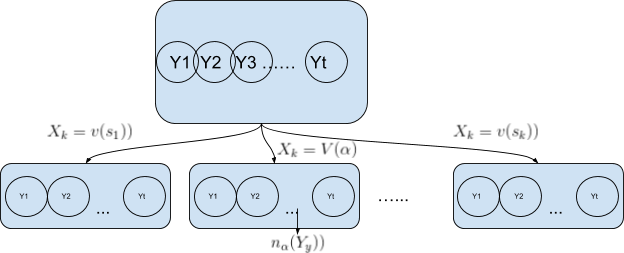
We first pickup a feature , e.g. an index k, ` 1 \leq k \leq n ` .
For that feature, we check how many categories are present for each possible value of the feature. For instance let us say that that we the feature takes ` s_{k} ` values. We create ` s_{k} ` subsets and each subset ` S_{ \alpha },1 \leq \alpha \leq s_{k} ` is populated with the amount of categories that are listed for values of ` X_{k}=V \left( \alpha \right) ` . Let us say that there will be ` n_{ \alpha } \left( y_{} \right) ` elements for each category ` Y_{y} ` in `Y`.
` n_{ \alpha } \left( y_{} \right) ` is therefore the amount of representatives of category ` Y_{y} ` in the subset defined by { ` X_{k}=V \left( \alpha \right) ` }.
So the initial set of categories is been partitioned into ` s_{k} ` subsets , each subset containing representants of categories from the initial subset.
Of course if `n(y)` is the number of elements in the original training set for a category `Y_{y} ` in Y , then ` n \left( y \right) = \sum _{1 \leq \alpha \leq s_{k}}^{}n_{ \alpha } \left( y_{} \right) `
The process is graphically represented in the following diagram:
Of course as we saw before this allows the computation of an information gain.
The initial entropy is `-\frac{n(Y_1)Log( \frac{n(Y_1)}{n_0})+ \ldots + n(Y_t)Log(\frac{n(Y_t)}{n_0})}{n_0}` .
Where ` n_{0}= \sum _{y=1}^{t}n \left( Y_{y} \right) ` is the total number of representatives of ` Y` .
The final entropy is `\frac{1}{n_{0}} \sum _{ \alpha =1}^{ \alpha =s_{k}}n_{ \alpha }E \left( S_{ \alpha } \right) `
Where ` n_{ \alpha } ` is the cardinal of ` S_{ \alpha } ` and ` E \left( S_{ \alpha }) ` is the entropy of ` S_{ \alpha }` .
We also have:
`n_{ \alpha }E \left( S_{ \alpha } \right) =- \sum _{y=1}^{t}n_{ \alpha } \left( Y_{y} \right) Log (\frac{n_{\alpha}(Y_y)}{n_\alpha}) `
So the information gain can be computed by the following formula:
`IG=-\frac{1}{n_{0}} \sum _{ \alpha =1}^{ \alpha =s_{k}} \sum _{y=1}^{t} n_{ \alpha } (Y_{y}) Log(\frac{n_{ \alpha } (Y_{y})}{n_\alpha}) + \frac{n(Y_1)Log( \frac{n(Y_1)}{n_0})+ \ldots + n(Y_t)Log(\frac{n(Y_t)}{n_0})}{n_0}`
Now since we have n ways to choose `k`, we can pick up the one that makes the Information gain maximal. This is obviously desirable.
Once we have done that we can iterate the same process for each subsets `S_{ \alpha }` . Since all these subsets correspond to a fixed value of ` X_{k}` we cannot reuse `k` and for each subsets generated, we won’t be able to use any feature vector that we used previously.
We continue the process until we reach a leaf, which means the entropy is maximal or there are no more available feature vectors.
Examples
We suppose that we have a training set with N=8 samples. We classify cars following 3 features: date of production , average speed, retail price The possible categories are cars manufacturers:
- Peugeot
- Volkswagen
- Ford
This can represent the average car models found in resellers such as Ford Mustang, Ford Transit, Fiat Uno, Peugeot 405 etc...
|
Date of production |
Speed |
Retail price |
Category |
|
Old |
High |
Expensive |
Ford |
|
Old |
Average |
Expensive |
Ford |
|
New |
High |
Average |
Peugeot |
|
New |
High |
Expensive |
Ford |
|
New |
Average |
Average |
Peugeot |
|
New |
Low |
Average |
Volkswagen |
|
Old |
Average |
Low |
Volkswagen |
|
Old |
Low |
Expensive |
Peugeot |
We can start to classify with the ‘date of production’, we will get this:
|
(FFPFPVVP) |
|
|
(FFVP) |
(PFPV) |
The entropy for the root node, in all cases is always = -(3Log(⅜)+ 3Log(⅜)+ 2Log(1/4))/8=0.47
The entropy for the subset generated with the date of production is
-2(2Log(2/4)+log(¼)+log(¼))/8=0.45
The information gain is therefore IG=0.47-0.45=0.02 which correspond to a relative gain of
1-0.45/0.47=4.2% which is really small.
Now let us try the ‘speed’, we get the following dataset:
|
(FFPFPVVP) |
||
|
(FFF) |
(FPV) |
(VP) |
The Entropy of the dataset is = -(0+3Log(⅓)+2Log(½))/8=0.25
Here we have a gain of 0.22 or a relative gain of around 47%.
Let us try finally the ‘Expensive’ feature:
|
(FFPFPVVP) |
||
|
(FFFP) |
(PPV) |
(V) |
The entropy of the dataset is = -( 3Log(¾)+Log(¼)+ 2Log(⅔)+Log(⅓)+0)/8=0.22
Here we have a gain of 0.25 and a relative gain of around 53%.
We will therefore choose the last dataset, the one created by considering the ‘Retail price’ feature’. It is just slightly better than the ‘Speed’ feature.
We then need to apply the algorithm to the 3 datasets. The last one, (V) is obviously a leaf. If a car is considered to have a low price, we will classify it as a Volkswagen (we didn’t try to be realistic in that example…let us say that V could have bee n a VAZ … or ВАЗ: Во́лжский автомоби́льный заво́д ) .
Let us work then with the set (FFFP). We have two features to consider: the date of production and the speed.recall that this is the set which is obtained with the value of Retail price=Expensive
|
Date of production |
Speed |
Retail price |
Category |
|
Old |
High |
Expensive |
Ford |
|
Old |
Average |
Expensive |
Ford |
|
New |
High |
Average |
Peugeot |
|
New |
High |
Expensive |
Ford |
|
New |
Average |
Average |
Peugeot |
|
New |
Low |
Average |
Volkswagen |
|
Old |
Average |
Low |
Volkswagen |
|
Old |
Low |
Expensive |
Peugeot |
|
(FFFP) |
|
|
(FFP) |
(F) |
The base Entropy is -(3Log(¾)+log(¼))/4=0.24
The entropy of the dataset is -(2Log(⅔)+log(⅓)+0)/4=0.20
We have a gain of 0.04 or a relative gain of 16%
If we consider the ‘Speed’ feature:
|
(FFFP) |
||
|
(FF) |
(F) |
(P) |
The entropy of the dataset is 0+0+0 so the gain is maximal = 100%
All nodes (datasets) are leafs.
Now we need to go back and consider the dataset with the value of Retail price=Average.
(PPV).
|
Date of production |
Speed |
Retail price |
Category |
|
Old |
High |
Expensive |
Ford |
|
Old |
Average |
Expensive |
Ford |
|
New |
High |
Average |
Peugeot |
|
New |
High |
Expensive |
Ford |
|
New |
Average |
Average |
Peugeot |
|
New |
Low |
Average |
Volkswagen |
|
Old |
Average |
Low |
Volkswagen |
|
Old |
Low |
Expensive |
Peugeot |
Since that dataset correspond also to fixed value of the data of production (=’New’), and therefore will create a gain of information =0, then we will consider the speed feature:
|
(PPV). |
||
|
(P) |
(P) |
(V) |
Here all nodes are leaf , we have a gain of information maximal of 100% and so we have completed our decision tree.
We display it in the following diagram.
|
(FFPFPVVP) |
|||||||
|
Value of ‘retail price’ ? |
|||||||
|
High |
Average |
Low |
|||||
|
(FFFP) |
(PPV) |
(V) |
|||||
|
Value of Speed feature? |
Value of Speed feature? |
|
|||||
|
High |
Average |
Low |
High |
Average |
Low |
||
|
(FF) |
(F) |
(P) |
(P) |
(P) |
(V) |
||
This is our ID3 classifier!
We can test it and ask him to classify the following input vector:
|
Date of production |
Speed |
Retail price |
|
New |
High |
Average |
The classifier predicts that it is a Peugeot.
Conclusion
The decision tree produced by the ID3 classifier is locally optimal in terms of Information gain but not necessarily globally optimal. Anyway ID3 classifiers can achieve good results. They are not greedy in terms of computing and they can therefore be used in systems with moderate or low computing power and resources.

References
Read more articles on Artificial Intelligence (2018 - today), by Martin Rupp, Dr. Ulrich Scholten, Iman Gowhari and more