


In this tutorial, we will have a detailed look at one of the most powerful classes of machine learning and Artificial Intelligence algorithms that exists: the Bayesian Classifiers.
A small introduction to Bayesian probabilities
Principles of Bayesian Classifiers and Bayesian Networks
Building our own Bayesian Classifiers
Powers and Weaknesses of Bayesian Classifiers

An introduction into Bayesian probabilities
Bayesian probabilities are conditional probabilities. They are a part of the Bayesian statistics named after their inventor, the mathematician Thomas Bayes[1].
The core principle is to compute the probability of an event knowing that another event has occurred. In other terms Bayesian probabilities explain how to compute the probability of A when you know that B with a probability of P(B)has realized, this is contained in the following formula (Bayes theorem) :
P(A|B)=P(B|A)*P(A)/P(B)
The formula reads literally “The probability of A to realize knowing that B has realized is equal to the product of the probability that B realizes knowing that A has realized by the probability that A realizes divided by the probability that B realizes”
That simple formula is a powerful engine to compute a lot of useful things in plenty of domains.
There are a lot of literature about Bayes Theorem in different forms, here we wish only to present what is needed for the reader to understand the Bayesian classifiers.
We are here interested in the Bayesian interpretation of the theorem:
P(A) represents the prior. That is to say the apriori belief that event A is true/ event A will realize.
P(A|B) represents the posterior, that is to say the belief A is true/A will realize taking the support that provides B into account.
P(B|A)/P(B) represents the support B provides to A. if that support is <1 then the support is negative, e.g the belief is A is lessened otherwise it is a positive support, the belief in A is enforced.
The Bayesian interpretation is the root of the Bayesian machine learning. This consists in believing some facts are true giving (anterior) facts realized.
We give here two examples of the power of Bayesian probabilities which often provides paradoxical solutions because our human brains evaluate in general very poorly such conditional probabilities.
Bayesian rule is often used in genetic engineering and in general in medicine. It is often a powerful tool for a doctor to make an opinion of take a decision.
Example #1
A particular virus has a base rate of occurrence of 1/1000 people. This means that on average 1 person over 1000 in the population will be affected by that virus.
It is essential to be able to detect the virus in the population before the incubation completes so to cure the infected people.
A governmental laboratory manufactured a test to detect that disorder. It has a false positive rate of 5%. This means that 5% of the time it says a given person has a disease, it is mistaken. We assume that the test never wrongly reports that a person is not infected (false negative rate of 0%).
In other words, if the test says a person is infected there is a 5% chance it is incorrect but if the test says a person is not infected, then this will be always correct.
Before a decision to start testing the population and producing massively test kits, the doctor in charge of the fight against virus is asked by the authorities the following question:
“What is the chance that a randomly selected person which have a positive result to the test is effectively infected by the virus?”
Most people would intuitively answer : 95% because as a matter of fact the test says wrongly that people are infected by the virus only 5% of the time.
The doctor being a highly trained specialist starts to use the Bayesian computations:
A is the event that a person has the disease.
B is the event that the person has a positive result to the test.
P(B|A) is the probability that a person which tests positive has the virus. This is what we need to compute. For that we need to compute P(A), P(B) and P(A|B).
It is easy to compute P(A) , this is 1/000= 0.001 (recall the virus infects on average one person over 1000 in the population)
P(A|B) is the probability that a person which has the disease will test positively, as we said the test has a false negative rate of 0%, so P(A|B)=1.
P(B) is the probability that a person in the population has a positive result to the test.
There are two independent ways that could happen:
- 1) The person has the disease
There are then a probability of 0.001 that a person has the disease
- 2) The person has not the disease and triggers a false positive
There is a probability of 0.999 that a person has not the disease and probability of 5%=0.05 that this person will trigger a false positive
Finally
P(B)=0.001 +(0.999)*0.05=0.051
We can compute P(B|A):
P(B|A)= 1*0.001/0.051=0.02
As a matter of fact the test will give on average correct results only 2% of the time, so it is highly inaccurate and an other test need to be manufactured!
The reality is that few people have the virus so the false positives even if they are “only” 5% are destroying the accuracy of the test but that fact is highly difficult for a human mind to apprehend.
Example #2
An international prestigious online insurance company must evaluate if they will accept a new customer or not
They know that on average 99% of their past customers which had Romanian citizenship submitted fraudulent claims. They also know that customers which are of Romanian citizenship accounted for 0.1% of their total fraudulent claims. Besides the amount of their romanian customers is 0.001%
The customer which is submitting the application is a very rich Romanian citizen, while apparently very risky, should the insurance company accept the new customer?
It is difficult to say because while it seems Romanian customers can not be trusted, they also account for a very small amount of fraudulent claim.
If A is the event that the customer is submitting a fraudulent claim and B the event that the customer is Romanian, then we need to compute P(B|A), this is the probability that a customer is romanian knowing a false claim has been issued by that customer.
P(B|A)=0.1%=0.001
A|B is the event that a romanian will submit a fraudulent claim, this is
P(A|B)=99%=0.99
P(A) is the overall risk with Romanian citizens and can be computed as such:
P(A)=P(B)*P(A|B)|P(B|A)
=0.00001*0.99/0.001=0.1%
One should think it is enough to look at P(A|B) and immediately decide to reject Romanian customers. This is not so simple. This does not reflect the impact to the overall risk.
As a matter of fact the company insurance would accept the customer because romanians does not significantly impact the overall risk which is acceptable for the insurance company. If we add other data such as gain expectations given the fortune of the new client, the decision may appear extremely logical given the risk policy of the company.
All these computations show the power of Bayesian logic especially because it unveils decisions to human people that their brains have difficulties to conceive.
Next we shall look to what is machine learning before we can understand how bayesian classifiers works.
What is Machine Learning
Machine learning refers to a class of algorithms - subset of the Artificial Intelligence algorithms class - where machines can make autonomous decisions based on a learning set which is eventually enforced all over the time. That learning set is used to make inferences regarding events or facts.
Supervised machine learning
Most machine learning algorithms belong to the supervised machine learning class.
In supervised learning, a set of inputs and outputs, the “training set” or “training examples” is known with relationships between both sets. Mainly a mapping from the inputs to the outputs.
From that Training set, the algorithm will build a model that will map new input to new outputs.
As an example, we can create an initial input set of 7 images and an initial output set of the 7 standard capitalized english alphabet letters A-G.
Input Set (Training set):
 |
.png?width=68&name=pasted%20image%200%20(1).png) |
.png?width=76&name=pasted%20image%200%20(2).png) |
.png?width=68&name=pasted%20image%200%20(3).png) |
.png?width=67&name=pasted%20image%200%20(4).png) |
.png?width=53&name=pasted%20image%200%20(5).png) |
.png?width=98&name=pasted%20image%200%20(6).png) |
Output Set:
| A | B | C | D | E | F | G |
In that example, a et of 27 images are mapped to letters (bytes or unsigned chars)
The algorithm will use that training set to map the following input:
.png?width=64&name=pasted%20image%200%20(7).png)
To one of the existing output. Here the right match is obviously ‘G’
Eventually this can be added to the learning set after some validation:
Input Set (Updated Training set):
|
|
|
|
|
|
|
|
Output Set:
| A | B | C | D | E | F | G | G |
Of course the algorithm would work with some data of the images, a n-vector. This may be for example : histogram, level of black and white pixels and similar data applied after various filters. This is how OCR usually works .
There are a lot of different strategies for machine learning. Usually a score function f is defined. Here it would be for example:
f(![]() ,’A’)=0.3
,’A’)=0.3
f(![]() ,’B’)=0.6
,’B’)=0.6
…
f(![]() ,’G’)=0.9
,’G’)=0.9
Then usually ![]() would be matched to the letter that maximizes the score function, e.g “G”.
would be matched to the letter that maximizes the score function, e.g “G”.
Here ![]() may be represented by the vector (X1,...,Xn) where Xi is the amount of pixels for the i^th tonal value (“image histogram”) . It may also be represented by a combination of such vector with other image characteristics.
may be represented by the vector (X1,...,Xn) where Xi is the amount of pixels for the i^th tonal value (“image histogram”) . It may also be represented by a combination of such vector with other image characteristics.
A fruit may be represented for instance by a color, a weight and a price.
The matching can also be represented by probability distributions and risk minimization.
There are two important types of unsupervised learning: Classifier learning and Regression learning.
Here we are only interested in the Classifiers.
Classifiers machine learning
The classifiers operates with outputs been restricted to a finite set of values (like in the previous aforementioned example with the letters).
Typical examples of Classifiers are :
- Artificial Neural Networks (ANN)
- Decision trees
- Support vector Machines
- Bayesian Classifiers
Next we detail the main topic of our article, how the Bayesian Classifiers and Bayesian Networks are working.
Principles of Bayesian Classifiers and Bayesian Networks
The Bayesian classifier is a learning machine which uses a finite fixed set of outputs , the labels or categories where the inputs, unknown must be classified. To do this, the Bayesian classifier use Bayesian logic, that is to say the correction of the prior belief that such input will fall into such category given support from additional events or information:
posterior (A|B)=prior(A) x support from additional facts (B|A/B)
Which can be formulated as :
posterior = prior x likelihood / evidence.
Here we defined likelihood as p(B|A) and evidence as p(B).
“Naive” Bayesian Classifier
First let us look as the most simple of all the Bayesian Classifiers , the “Naive” Bayesian Classifier.
The main idea behind such classifier is that we are given at the start the following conditional probabilities:
 k=1,...,m
Where .png?width=60&name=chart%20(1).png) are the available categories and
are the available categories and .png?width=99&name=chart%20(2).png) is the input vector to classify.
is the input vector to classify.
We can write:
.png?width=331&name=chart%20(3).png) k=1,...,m
k=1,...,m
The term P(X) is a normalizer constant in that sense that it does not depend on the m categories.  is easy to compute, it is the proportion of the whole dataset which is classified in the category Ck.We can compute
 -1.png?width=74&name=chart%20(2)-1.png) by considering that it is proportional to the joint probability model
by considering that it is proportional to the joint probability model -1.png?width=67&name=chart%20(2)-1.png) and then we may apply the following rule chain:
and then we may apply the following rule chain:
 k=1,...,m
And then finally by iterating n times that chain rule:
-2.png?width=711&name=chart%20(1)-2.png)
The components of X are supposed to be all independants and by the so-called “naive” hypothesis:
-2.png?width=276&name=chart%20(2)-2.png)
Here we must explain two aspects:
- It is not trivial why a conditional probability is suddenly “transformed” into a joint probability . In fact
 by the probability chain rule, so the both quantities - seen as depending only on X - are proportionals
 - It is also not trivial what the “naive” hypothesis means and why it is called “naive”.
The components of X are supposed to be all independants - this is where the naivety is, so as a consequence, the condition that we have a realization of a value for one of the components of X should not depend on the realization of the others components of X but only on the realization of the categories.
From there, we can compute our model:
.png?width=339&name=chart%20(1).png) k=1,...,m
k=1,...,m
And Z is a scaling factor equal to:
.png?width=275&name=chart%20(2).png)
These equations are the basis of the “Naive” Bayesian classifiers which are among one of the most powerful classifiers that exists.
Usually the decision to classify, that is to say to create a mapping between the input vector X and one of the output categories will be done by the Maximal a Posteriori (MAP) but it can also be done via the Maximal Likelihood (MLE)
MAP decision making
We classify ![]() as
as ![]() such as:
such as:
.png?width=173&name=chart%20(4).png)
where:
.png?width=177&name=chart%20(5).png)
MLE decision making
We classify ![]() as
as ![]() such as:
such as:
where:
.png?width=175&name=chart%20(7).png)
Both approaches have their pros and cons. MLE and MAP are widely used techniques in machine learning.
We have now all the material needed to program concrete Bayesian Classifiers.
We will explain the principles of the others type - more sophisticated - of Bayesian Classifiers but we will restrict implementations to Naive ones for the sake of simplicity.
Bayesian classifiers may use naive models but with the assumption that the probability will follow a normal distribution. The normal distribution is then computed by the estimation of the mean and variance parameters from each category in the existing dataset. Same may be done with multivariate Bernoulli and other probability laws.
Example #3
Here we present a basic example of Bayesian naive classification.
We wish for a robot that works in a warehouse to classify/sort vegetables which are unloaded from a truck to a conveyor belt . The robot has several sensors that will provide him information but no video camera- just the ability to get the dominant color of the vegetable. We use the following input vector X:
- Color (yellow,brown,white,red,orange,dark,green)
- Big size(XXL)
- Average size (X)
- Mall size (S)
- Big weight (W+)
- Average weight (W)
- Small weight (W-)
The space of the inputs is a finite space with 63 possible values (7*3*3).
At the start the vegetables are manually calibrated, there are different quantities and for each quantity the result of the calibration is noted in a table as such:
|
|
Qty |
Y |
B |
W |
R |
O |
D |
G |
XXL |
X |
S |
W+ |
W |
W- |
|
|
700 |
20 |
0 |
0 |
600 |
70 |
0 |
10 |
2 |
623 |
75 |
2 |
580 |
118 |
|
|
45 |
0 |
0 |
0 |
45 |
0 |
0 |
0 |
0 |
5 |
40 |
0 |
5 |
40 |
|
|
34 |
0 |
0 |
0 |
34 |
0 |
0 |
0 |
0 |
3 |
31 |
0 |
0 |
34 |
|
|
25 |
1 |
2 |
0 |
0 |
0 |
0 |
22 |
18 |
7 |
0 |
1 |
24 |
0 |
|
|
100 |
8 |
0 |
0 |
0 |
92 |
0 |
0 |
70 |
30 |
0 |
100 |
0 |
0 |
|
|
18 |
18 |
0 |
0 |
0 |
0 |
0 |
0 |
10 |
8 |
0 |
1 |
17 |
0 |
|
|
5 |
0 |
0 |
0 |
0 |
0 |
0 |
5 |
5 |
0 |
0 |
0 |
5 |
0 |
|
|
300 |
0 |
300 |
0 |
0 |
0 |
0 |
0 |
20 |
200 |
80 |
15 |
240 |
45 |
|
|
400 |
0 |
0 |
0 |
0 |
400 |
0 |
0 |
0 |
400 |
0 |
0 |
400 |
0 |
|
|
30 |
0 |
1 |
25 |
0 |
0 |
4 |
0 |
30 |
0 |
0 |
30 |
0 |
0 |

.png?width=100&name=pasted%20image%200%20(1).png)
.png?width=100&name=pasted%20image%200%20(2).png)
.png?width=100&name=pasted%20image%200%20(3).png)
.png?width=100&name=pasted%20image%200%20(4).png)
.png?width=100&name=pasted%20image%200%20(5).png)
.png?width=100&name=pasted%20image%200%20(6).png)
.png?width=100&name=pasted%20image%200%20(7).png)
.png?width=100&name=pasted%20image%200%20(8).png)
.png?width=100&name=pasted%20image%200%20(9).png)
The robot is then loaded with the following dataset, the conditional probabilities are computed from the frequencies. Read the case (X,F) : “probability of feature F given that it is a vegetable X”.
Examples:
Probability it is green, given it is a tomato = 0.01=1%
Probability it is green, given it is a lettuce = 0.88=88%
Probability it is of small size (S) given it is a banana= 0.00=0%
|
|
Y |
B |
W |
R |
O |
D |
G |
XXL |
X |
S |
W+ |
W |
W- |
|
|
0.03 |
0.00 |
0.00 |
0.86 |
0.10 |
0.00 |
0.01 |
0.00 |
0.89 |
0.11 |
0.00 |
0.83 |
0.17 |
|
|
0.00 |
0.00 |
0.00 |
1.00 |
0.00 |
0.00 |
0.00 |
0.00 |
0.11 |
0.89 |
0.00 |
0.11 |
0.89 |
|
|
0.00 |
0.00 |
0.00 |
1.00 |
0.00 |
0.00 |
0.00 |
0.00 |
0.09 |
0.91 |
0.00 |
0.00 |
1.00 |
|
|
0.04 |
0.08 |
0.00 |
0.00 |
0.00 |
0.00 |
0.88 |
0.72 |
0.28 |
0.00 |
0.04 |
0.96 |
0.00 |
|
|
0.08 |
0.00 |
0.00 |
0.00 |
0.92 |
0.00 |
0.00 |
0.70 |
0.30 |
0.00 |
1.00 |
0.00 |
0.00 |
|
|
1.00 |
0.00 |
0.00 |
0.00 |
0.00 |
0.00 |
0.00 |
0.56 |
0.44 |
0.00 |
0.06 |
0.94 |
0.00 |
|
|
0.00 |
0.00 |
0.00 |
0.00 |
0.00 |
0.00 |
1.00 |
1.00 |
0.00 |
0.00 |
0.00 |
1.00 |
0.00 |
|
|
0.00 |
1.00 |
0.00 |
0.00 |
0.00 |
0.00 |
0.00 |
0.07 |
0.67 |
0.27 |
0.05 |
0.80 |
0.15 |
|
|
0.00 |
0.00 |
0.00 |
0.00 |
1.00 |
0.00 |
0.00 |
0.00 |
1.00 |
0.00 |
0.00 |
1.00 |
0.00 |
|
|
0.00 |
0.03 |
0.83 |
0.00 |
0.00 |
0.13 |
0.00 |
1.00 |
0.00 |
0.00 |
1.00 |
0.00 |
0.00 |
Some vegetables can be uniquely identified by a color , for example only potatoes are brown, so if the classifier will see a brown vegetable, it will conclude that it is probably a potato.
That table is the initial dataset of the naive Classifier. It will evolve with time as the robot ( more precisely the AI in the robot’s program ) will add new knowledge to the previous dataset.
Now the robot receives this vegetable from the conveyor belt:
.png?width=58&name=pasted%20image%200%20(10).png)
This is a cherry tomato. small, red, compact. It has the following features:
X=(R,S,W)=(0,0,0,1,0,0,0,0,0,1,0,1,0)
Note that most of the cherry tomatoes in the dataset have the features X=(R,S,W-)
But that one is a relatively compact cherry tomato.
To classify that new vegetable, the classifier must compute the 10 values:

…
-1.png?width=245&name=chart%20(1)-1.png)
-1.png?width=288&name=chart%20(2)-1.png)
And classify the new vegetable in the category that will give the maximal value.
Here we are faced with one of the main issues when dealing with Bayesian classifiers, the zero probabilities. Indeed since vegetables cannot be red and green for example, one of the probabilities in the product is always 0. For this we can either smooth the data, by transforming 0 into a tiny amount, smaller than all the present probabilities, 0.001 for example or changing our input vector.
Here we will change our input vector as such:
|
Y |
B |
W |
R |
O |
D |
G |
XXL |
X |
S |
W+ |
W |
W- |
|
1 |
2 |
3 |
4 |
5 |
6 |
7 |
1 |
2 |
3 |
1 |
2 |
3 |
So that the input vector is coded as (4,3,2).

-2.png?width=265&name=chart%20(1)-2.png)
-2.png?width=464&name=chart%20(2)-2.png)
-1.png?width=239&name=chart%20(3)-1.png)
We need to do these computations for the 8 categories that are left , we finally end with the following values[2]:
|
Vegetable |
F(Vegetable) |
|
|
0.078 |
|
|
0.098 |
|
|
0 |
|
|
0 |
|
|
0 |
|
|
0 |
|
|
0 |
|
|
0 |
|
|
0 |
|
|
0 |
The value is null for the strawberry because there isn\'t a strawberry of weight W. All the others vegetables are not red so we get as well a null value.This can be read “ If it’s red , it’s not going to be a lettuce” because it hasn\'t seen any red lettuce so far and so on …
We can smooth the table so to avoid null values by adding one sample in every category. Yet the MLE will stay very small so instead of the zero values we will have very tiny numbers and here this will not change the end result anyway.
As a matter of fact, the robot will rightly classify the cherry as a cherry tomato because it has a higher value to the MLE decision.
Note that in general the robot may have a hard time distinguishing cherry tomatoes from strawberries so other features may have to be added like eventually more tone of color or more weight or more sizes.
This example,while very simple, demonstrates how the naive Bayesian classifiers works.
Bayesian Classifiers Networks
The “naive” assumption that there is independence of the vector data of the input X is often, in many applications, unrealistic Therefore to tackle that problem, Bayesian networks were invented.
The principle is to represent relationship between the vector component of X, eg the  by a unidirectional arrow. Therefore a graph will represent the components
 -3.png?width=86&name=chart%20(1)-3.png) which must be taken into account into the overall computations of the MLEs or MAPs.
which must be taken into account into the overall computations of the MLEs or MAPs.
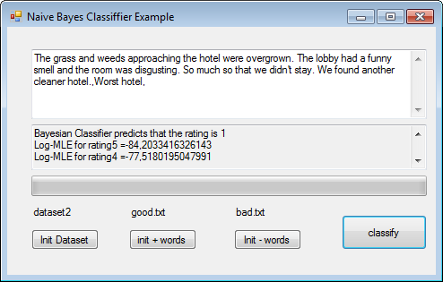
We seek to classify fraud data for an insurance company.
Here we consider a vector X made of 5 components:
-3.png?width=22&name=chart%20(2)-3.png) : Town
: Town-2.png?width=23&name=chart%20(3)-2.png) : Net Income
: Net Income-1.png?width=23&name=chart%20(4)-1.png) : Age
: Age-1.png?width=23&name=chart%20(5)-1.png) : Profession
: Profession-1.png?width=23&name=chart%20(6)-1.png) : Education
: Education
Of course the components are not independents. We have relationships between the town (and therefore the country) and the income. The income depend also of the age, profession and education. Besides, age, education and profession are linked.
This means that we must take into account the proportions P(income|Town) , P(income|age), P(income|profession), P(income|education), P(profesion|age) and P(education|profession).
Here we wish not to elaborate on the Bayesians networks because their description may be quite complex. Nevertheless, they do not always perform better than the Naive ones as surprising as it may seem.
Building our own Bayesian Classifiers
There are a lot of areas where Classifiers can be good and useful. We will start by trying to build a classifier for detecting emotions in text, using C#.
We will consider only english language for the input text.
Example #4
We will get the training data from a website where users give their opinions about hotels.
Usually a hotel is been given a note which reflect a feeling. A sentiment. For example:
1/5= very negative (depict, hate) 😠
2/5= negative (depict) 😡
3/5= neutral (indifference)😐
4/5 = positive (like)😊
5/5 = very positive (like, love)😃
The space of inputs will be the total amount of words present in the dataset, except the articles, pronouns “the”, “she”,”he” , “we”, “they”, and equivalent word such as “is”, “at” etc… The words must be present in the english dictionary so that excludes as well people’s names company\'s names etc…
Once the dataset created, usually by data mining using web scrapers, the classifier should be able to classify an english text into the above 5 categories.
Here we will use a free dataset from https://data.world[3] . This consists of a database of hotels reviews.
We get about 35k of review, most in english about different hotel. Of course, we are not interested by the hotels in themselves but only the mapping notation → review.
Here we present an example of the dataset, after we clean it :
As example here of what is a very negative review 1/5:
😠 "This was a true nightmare. The add stated it was oceanfront, it wasnt! the front door would not lock. It had gray duct on the lock section, which was painted it over. It appeared to be a place for squatters. It was not safe. The furniture was old, outdated and it smelled. And we couldn\'t get a refund!"
The review contains only negative terms: “nightmare”, “wasnt”, “not”, “old”, “outdated”, “smelled”, “couldn’t”, “refund” which is consistent with a very negative opinion of 1/5.
Opposingly here is how a positive review 4/5 looks like:
😊 "The Hotel staff were very friendly and accommodating. The rooms were fine. There was a mini fridge, microwave, hair dryer, and ironing board/iron. However the showers were awful. The water would get scalding hot and then ice cold. At first we thought it was because everyone was returning from the beach but it continued. The Hotel is in a great location-5 block walk to beach, boardwalk, restaurants, shops and entertainment. The pool was nice with not many people there. All in all experience was fine-I would probably return because the price was good and the only bad thing was the showers."
Here we see how the combination of positive “very friendly” , “fine”, “nice”, “great”, “fine”, “good” and negative opinion “awful”, “bad” leads to a positive review but with ‘mixed’ feelings.
The positive terms are in proportion of 3 to 1 to the negative terms and this is consistent with the 4/5 notation.
Our program needs first to read the dataset, then to build the table of conditional probabilities and finally implement the MLE method to classify a new text.
As we mentioned we will need to filter the input reviews first by removing numbers , pronouns, articles etc… and everything which is not in a reference english dictionary ( so we should get rid of foreign languages words as well) . In fact, as a parallel approach, we will even also filter much more and restrict ourselves to a dictionary of good/bad emotions. This is a very popular request in AI, so we have no issue to locate such files.
We take the list at https://gist.githubusercontent.com/mkulakowski2/4289437/raw/1bb4d7f9ee82150f339f09b5b1a0e6823d633958/positive-words.txt for our positive words
And the list at https://gist.githubusercontent.com/mkulakowski2/4289441/raw/dad8b64b307cd6df8068a379079becbb3f91101a/negative-words.txt for our negative words.
Our input vector X will therefore have
- A maximum of 4783+2007=6790 components consisting of all the words from both dictionaries in the parallel approach
We will compare both approaches and check which one seems the most reliable. We can also combine both classifiers!
Note that filtering and classifying is very common in data analysis. For example devices that are doing brain-machine interfaces are using a great lot of such filters and classifiers, combined togethers in relatively complex “designed” diagrams, so to process “mind orders” from an EEG helmet.
Here is the code that loads the “raw” dataset and computes the conditional probabilities :
string f_ = dialog.FileName;
string[] datas = File.ReadAllLines(f_);
//expecting note,text
label3.Text = Path.GetFileName(f_);
int max = datas.Length;
textBox2.Text = "initializing dataset," + max + " records \r\n";
progressBar1.Maximum = max + 10;
//getting rid of numbers, everything which is not in english dictionary
int c1 = 0;
foreach (string data in datas)
{
c1++;
progressBar1.Value = c1;
System.Windows.Forms.Application.DoEvents();
try
{
string n = data.Split(new char[] { \',\' })[0];
Int16 n_ = Int16.Parse(n);
if ((n_ < 1) || (n_ > 5))
continue;
string review = data.Split(new char[] { \',\' })[1];
foreach (string good in Positive)
{
//amount of occurence of the word in the review
// Int16 c=(Int16) Regex.Matches(data, bad).Count;
Int16 c = (Int16)review.Split(new String[] { good }, StringSplitOptions.None).Length;
// if (c > 1)
c--;
if (!(word_count[n_].ContainsKey(good)))
word_count[n_][good] = 0;
word_count[n_][good] += c;
review_totals[n_] += c;
}
foreach (string bad in Negative)
{
//amount of occurence of the word in the review
// Int16 c=(Int16) Regex.Matches(data, bad).Count;
Int16 c = (Int16)review.Split(new String[] { bad }, StringSplitOptions.None).Length;
// if (c > 1)
c--;
if (!(word_count[n_].ContainsKey(bad)))
word_count[n_][bad] = 0;
word_count[n_][bad] += c;
review_totals[n_] += c;
}
}
catch (Exception ex)
{
}
}
}
textBox2.Text += "dataset processed \r\n";
//we remove words which have no match anywhere
foreach (string good in Positive)
{
int p = 0;
for (Int16 i = 1; i < 6; i++)
{
if (!(word_count[i].ContainsKey(good))) word_count[i][good] = 0;
p += word_count[i][good];
}
if (p > 0)
inputs.Add(good);
}
foreach (string bad in Negative)
{
int p = 0;
for (Int16 i = 1; i < 6; i++)
{
if (!(word_count[i].ContainsKey(bad)))
word_count[i][bad] = 0;
p += word_count[i][bad];
}
if (p > 0)
inputs.Add(bad);
}
textBox2.Text += "Dataset cleaned: "+inputs.Count+" vectors remaining \r\n";
for (Int16 i = 1; i < 6; i++)
{
foreach (string x in inputs)
{
//smoothing ... every words appears one times!
// word_count[i][x]++;
bayesian_probas[i][x] = decimal.Divide(word_count[i][x], review_totals[i]);
}
}
Once computed by our program, our final dataset looks like that:
|
rating/ |
accessible |
adequate |
advanced |
advantage |
... |
|
1 |
0,0010548523206751054852320675 |
0 |
0 |
0 |
... |
|
2 |
0 |
0,001700680272108843537414966 |
0 |
0 |
.. |
|
3 |
0,0007278020378457059679767103 |
0,0029112081513828238719068413 |
0,0007278020378457059679767103 |
0 |
... |
|
4 |
0,0011952191235059760956175299 |
0,0011952191235059760956175299 |
0 |
0 |
... |
|
5 |
0,0002790178571428571428571429 |
0,0005580357142857142857142857 |
0 |
0,0011160714285714285714285714 |
... |
Each case in the table is, like always, P(rating=y | x_i>0) and we have only 755 coordinates for each input after removing useless inputs.
In order to address the probability that input coordinate x contains n times a given word , we can estimate that probability by a Gaussian variable:

Where ![]() and
and ![]() are respectively the mean and variance which are computed from the sample inputs.
are respectively the mean and variance which are computed from the sample inputs.
We may also count the amount of samples with x_i=n for a rating y
Here we will restrict ourselves to the fact that the word is not present (value = 0) or present at least one time (value = 1) This is of course less accurate.
One other issue is the smoothing. We cannot really add one sample to every input (Laplace smoothing) because we have 754 vectors and therefore most occurrences of words are scarce, most vectors values are 1 or 2. So adding one sample would change all the probabilities dramatically.
There are various others smoothing methods such as Jelinek-Mercer Smoothing, Dirichlet Smoothing, etc… but here we want to stay a simple as possible so we will just decide that even if the classifier hasn’t seen a word in a review for a given rating(1-5) there is still a non-null probability - yet very small - that if it meets that word, then the review will belong to that given rating.
As for the “very small” probability, we will decide empirically that it is 1/100 of the smallest probability for all the non-null probability for that given rating. In other words:
-3.png?width=651&name=chart%20(3)-3.png)
Here is the code that does the smoothing:
//smoothing
foreach (string x in inputs)
{
Decimal pmin = 0;
Decimal p2 = 0;
for (Int16 i = 1; i < 6; i++)
{
if (bayesian_probas[i][x] == 0)
continue;
pmin = bayesian_probas[i][x];
if( (p2 < pmin)&&(p2>0))
pmin = p2;
p2 = pmin;
}
Decimal pzero = Decimal.Divide(pmin, 100);
for (Int16 i = 1; i < 6; i++)
{
if (bayesian_probas[i][x] == 0)
bayesian_probas[i][x] = pzero;
}
}
After the smoothing we get the new probability dataset table:
|
rating/ |
accessible |
adequate |
advanced |
advantage |
... |
|
1 |
0,0010548523206751054852320675 |
0,0000055803571428571428571429 |
0,0000072780203784570596797671 |
0,0000111607142857142857142857 |
... |
|
2 |
0,0000027901785714285714285714 |
0,001700680272108843537414966 |
0,0000072780203784570596797671 |
0,0000111607142857142857142857 |
.. |
|
3 |
0,0007278020378457059679767103 |
0,0029112081513828238719068413 |
0,0007278020378457059679767103 |
0,0000111607142857142857142857 |
... |
|
4 |
0,0011952191235059760956175299 |
0,0011952191235059760956175299 |
0,0000072780203784570596797671 |
0,0000111607142857142857142857 |
... |
|
5 |
0,0002790178571428571428571429 |
0,0005580357142857142857142857 |
0,0000072780203784570596797671 |
0,0011160714285714285714285714 |
... |
Now we are in a position of computing the MLEs and classify any incoming English text !
The MLE will therefore compute the quantities:

For the ratings y=1 to x=5.
There is a point we must clarify. How do we compute the probability that a review will belong to a given rating category if a given word does not appear ? We know that the probability that a review belongs to the ratings ‘1’ (very negative) if it contains the term “accessible” is given by p= 0,0010548523206751054852320675 but what is the probability that a review belongs to the ratings ‘1’ if it does not contain the term ‘accessible’ ? well this is just p’=1-p=1-0,0010548523206751054852320675.
Our next problem will be to compute MLEs with 754 factors and get enough precision.
We can easily fix the issue by computing the Log-MLE, since the logarithm is strictly increasing function, a maximum of the MLE is a maximum of the log-MLE.
So we need to compute:
-5.png?width=651&name=chart%20(1)-5.png)
Here is the code that will compute the Log-MLE and classify:
string text = textBox1.Text;
if (text.Equals(""))
{
MessageBox.Show("no text input!", "error", MessageBoxButtons.OK, MessageBoxIcon.Error);
return;
}
//get frequency of input words
Dictionary<String, Int16> Bayesians_input = new Dictionary<String, Int16>();
foreach (string x in inputs)
{
Int16 c = (Int16)text.Split(new String[] { x }, StringSplitOptions.None).Length;
c--;
if (c > 0)
Bayesians_input[x] = 1;
else
Bayesians_input[x] = 0;
}
Double[] MLE = new Double[6];
//compute the MLE
for (Int16 i = 1; i < 6; i++)
{
Double p = 0;
foreach (string x in inputs)
{
if (Bayesians_input[x] == 1)
p += Math.Log( (double) bayesian_probas[i][x]);
else if (Bayesians_input[x] == 0)
p += Math.Log((double)(1-bayesian_probas[i][x]));
else
{
MessageBox.Show("error in computation word="+x+" input="+ Bayesians_input[x], "error", MessageBoxButtons.OK, MessageBoxIcon.Error);
return;
}
}
MLE[i]=p;
textBox2.Text = "Log-MLE for rating" + i + " =" + p + " \r\n" + textBox2.Text;
}
Int16 imax = 1;
Double pmax = 0;
Double p2 = 0;
for (Int16 i = 1; i < 6; i++)
{
p2 = MLE[i];
if ((p2 > pmax)||(pmax == 0))
{
pmax = p2;
imax = i;
}
}
textBox2.Text="Bayesian Classifier predicts that the rating is "+imax+ "\r\n" + textBox2.Text;
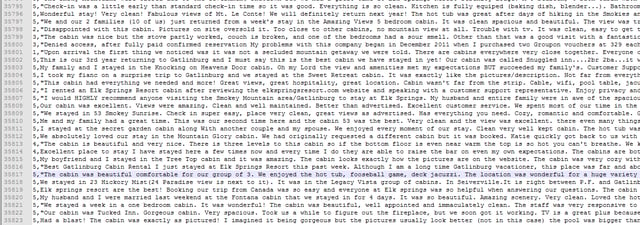
Now we can enjoy testing our small tool.
We first train it with a small subset of the database, around 2,000 records.
It predicts rightly very negative feedback..
-1.png?width=494&name=pasted%20image%200%20(1)-1.png)
However it will wrongly predict 3(neutral) when it is 2(negative)
-1.png?width=494&name=pasted%20image%200%20(2)-1.png)
Usually the Classifier will predict correctly , for example:
-1.png?width=494&name=pasted%20image%200%20(3)-1.png)
Here we see that it can predict a very positive feeling even if the world nightmare referring to another hotel is contained in the review!
We will next train our classifier with ALL the reviews and it will take a while to load dataset, around 10 minutes!
-1.png?width=499&name=pasted%20image%200%20(4)-1.png)
Our goal will be to check what the classifier can say when we type freely a text to give our opinion about anything, not just a hotel, like a tweet for instance:
-1.png?width=499&name=pasted%20image%200%20(5)-1.png)
That tweet is classified as “very negative”..
-1.png?width=499&name=pasted%20image%200%20(6)-1.png)
That tweet is also categorised as “very negative” and the next one as “very positive”.
-1.png?width=499&name=pasted%20image%200%20(7)-1.png)
But it detects a “neutral” text as a positive text:
-1.png?width=499&name=pasted%20image%200%20(8)-1.png)
We have built a working classifier which is able to detect negative or positive emotions in an english text.
Of course our classifier is very primitive and mainly built for the purpose of demonstrating how to implement a Bayesian classifier. For instance it cannot understand things like “not good=very bad” , “not bad=relatively good” and have to be trained to make the difference. Yet the Classifier works and could be used - for instance - to generate automatically a rating 1-5 from a customer feedback. Imagine a hotel website having to import a database of client’s feedback without any ratings into a database where ratings are mandatory and will be displayed on the website .
To complete let us see where we can find in everyday’s life, Bayesian Classifiers.
Existing Bayesian Classifiers
Bayesian Classifiers are everywhere but you probably never noticed them!
Spam Detection
Systems like SpamAssassin are using Bayesian Classifiers
The Spam detection systems works similarly with our negative/positive emotions classifier, it uses a learning set of keywords which are usually found in spam but also words which are usually not found in spam.
Spam training archive can be found at: http://artinvoice.hu/spams/
The SpamAssassin anti-spam has also auto-learning features which means it will increase its dataset with the time.
Anti-Fraud
Anti-Fraud is a very important important domain of Bayesian Classifiers. In insurance, risk management in general and to prevent credit-card fraud (card-not-present fraud )
There are good introductions to such topic in the following paper:
Using Bayesian Belief Networks for credit card fraud detection
Emotion Detection
As we have seen emotion detection can be realized with Bayesian classifiers.
They are used by various internet companies working in social networks, online marketing etc…
Man-Machine Interface
One surprising area of use of Bayesian Classifiers is man-machine interaction. Brain-Machine interfaces for example where what the user is thinking is to be interpreted by the machine.
Decision systems
As we also saw in the beginning of this article, Bayesian Classifier can also be used for computer-based decision, especially in medicine, genetic engineering , military systems etc…
There are many more areas where the Bayesian Classifiers are used everyday, we only wanted to give a few examples here.
Powers and Weaknesses of Bayesian Classifiers
Finally let us conclude with the pros and cons of such systems. Using Bayesian Classifier in a system is known to greatly reduce false positive and false negative but it may involve a really huge learning set. As we also saw Bayesian Classifiers needs empirical smoothing and the smoothing technique greatly depends one each case.
Bayesian Classifiers are powerful but they may also behave in a weird way…lack of data or lack of access to the right data may be the first cause of badly implemented Classifiers. Do not expect a miracle, a poorly trained classifier will behave badly.

Other Sources and References
- More articles on artificial intelligence (2019 - today), by Martin Rupp, Ulrich Scholten, Dawn Turner and more
- LEARNING ALGORITHMS FOR CLASSIFICATION: A COMPARISON ON HANDWRITTEN DIGIT RECOGNITION (2000), by Yann LeCun, L. D. Jackel & al, AT&T Bell Laboratories
- [1] ✝1701?–1761
- [2] P should be noted as P~ in the numerical computations because it is an estimate of the probability P, here for the sake of simplicity we keep the same notation.
- [3] https://download.data.world/datapackage/datafiniti/hotel-reviews